[Paper Review] Image Super-Resolution via Iterative Refinement (SR3)

지금 리뷰할 논문은 Diffusion을 이용한 Super-Resolution 방법 중 기초가 되는 SR3에 관한 논문이다.

해당 논문은 아래의 링크에서 확인할 수 있다.

Image Super-Resolution via Iterative Refinement

We present SR3, an approach to image Super-Resolution via Repeated Refinement. SR3 adapts denoising diffusion probabilistic models to conditional image generation and performs super-resolution through a stochastic denoising process. Inference starts with pure Gaussian noise and iteratively refines the noisy output using a U-Net model trained on denoising at various noise levels. SR3 exhibits strong performance on super-resolution tasks at different magnification factors, on faces and natural images. We conduct human evaluation on a standard 8X face super-resolution task on CelebA-HQ, comparing with SOTA GAN methods. SR3 achieves a fool rate close to 50%, suggesting photo-realistic outputs, while GANs do not exceed a fool rate of 34%. We further show the effectiveness of SR3 in cascaded image generation, where generative models are chained with super-resolution models, yielding a competitive FID score of 11.3 on ImageNet.

arXiv.orgChitwan Saharia

참고한 글은 아래와 같다.

[논문리뷰] Image Super-Resolution via Iterative Refinement (SR3)

SR3 논문 리뷰

전생했더니 인공지능이었던 건에 대하여JiYeop Kim

SR3 - Diffusion Model 논문 리뷰

SR3 논문의 핵심 내용을 리뷰합니다. 먼저 기존 방법의 문제점을 살펴봅니다. 이어서 이를 해결하기 위한 SR3의 제안 방법을 살펴봅니다. 마지막으로 성능 비교 실험을 통해 SR3의 효과를 확인합니다.

FFightingFfightingseok

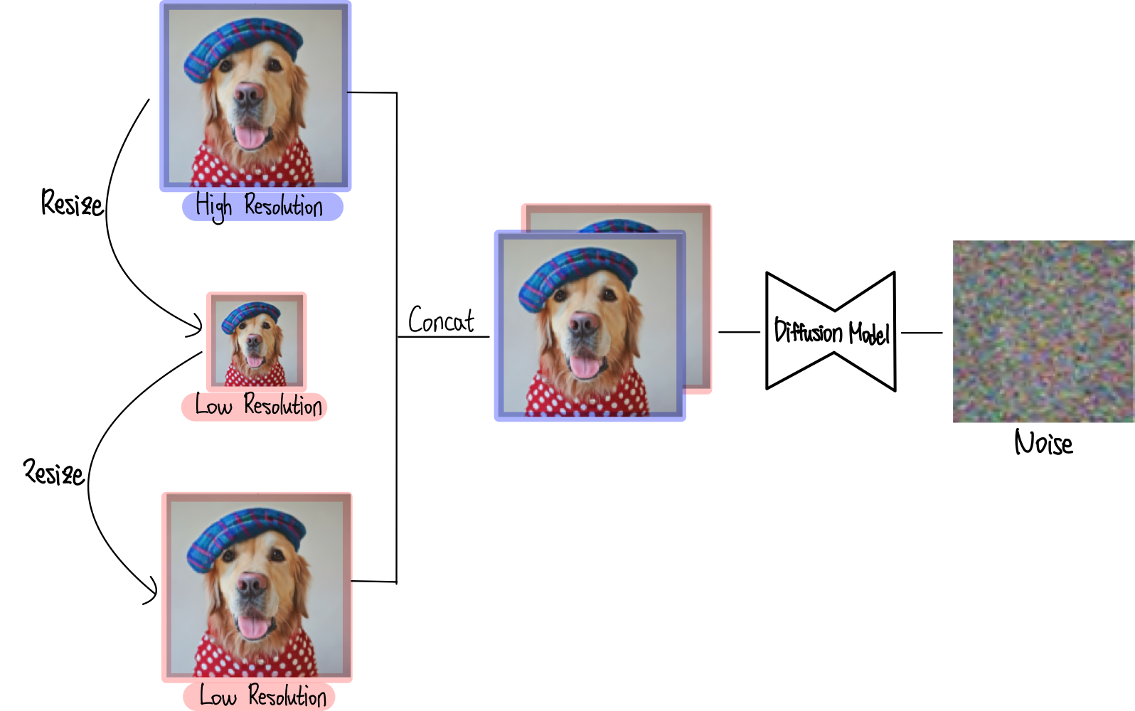
0. Abstract

저자들은 SR3라는 image Super-Resolution via Repeated Refinement라는 접근을 소개한다.

SR3는 conditional image generation을 위해 DDPM(Denosing Diffusion Probabilistic Model)을 이용하며,

stochastic iterative denoising process를 통해 super-resolution을 수행한다.

SR3 Model의 output 생성은 다음과 같이 이루어진다:

pure Gaussian Noise에서 시작하여, various noise level에서 trained U-Net(Training)을 이용하여 iteratively하게 noise output $\epsilon$을 refine(Sampling)한다.

전반적인 모델의 동작과정은 다음과 같다.

SR3 Model은 on faces나 natural images를 대상으로 다양한 magnification factor에 대한 super-resolution task에 있어서는 강한 performance를 보인다.

• human evaluation: standard 8x face super-resolution on CelebA-HQ compared with SOTA GAN methods
  • SR3: fool rate close to 50%
  • SOTA GAN: fool rate of 34%

• Cascaded image generation: super-resolution model들과 chained
  • ImageNet: FID score of 11.3

1. Introduction

Super-Resolution은 LR(Low-Resolution)을 condition으로 주었을 때, HR(High-Resolution)의 distribution (or $\text{HR} - \text{LR}$)을 modeling하는 Conditional Image Generation Task의 일종이다.

Single Image Super-Resolution은 다음의 I/O을 따른다:

• Input: low-resolution image
• Output: high-resolution image

이러한 Super-resolution은 image-to-image translation task의 일종이며, inverse problem 중 하나이다.

Inverse Problem


다음과 같은 Linear한 Noise Model이 있다고 하자.


$$g(x, y) = H(f(x, y)) + \eta(x, y)$$


- $g(x, y)$: camera 취득 영상 (vector)

- $f(x, y)$: 육안으로 보고있는 simulator (vector)

- $H$: 왜곡되는 Degradation 과정 (Matrix)

- $\eta(x, y)$: Noise (vector)


이때, $f$는 원인이고 $g$는 결과이므로


$f \rightarrow g$: forward process (Degradation)

$f \leftarrow g$: backward process

$\hat{f} \leftarrow g$: inverse problem (Restroation)

즉, 결과(low-resolution image)인 $g$로부터 원인(high-resolution image)인 $f$를 예측해야 하므로, Super-Resolution Task는 inverse problem의 종류 중 하나이다.

그러나, 이러한 Super-Resolution은 다음의 사항들로 인해 challenging하다:

• 하나의 input(결과)에 대하여 다수의 output(원인)이 가능하다.
• 주어진 input에 대한 output의 conditional distribution이 간단한 parametric distribution을 따르지 않는다.
  • e.g. multivariate gaussian과 같은 간단한 분포 X

기존에도 Deep Generative Model들을 이용하여 super-resolution과 같은 conditional task에 활용하는 경우가 있었다.

그러나 각 모델들은 다음의 이유로 한계점들이 있었다:

• GAN: model collapse와 optimization instability를 다루기 위해 designed regularization과 optimization trick들을 매우 조심히 설정해야 한다

• Autoregressive Models: HR image generation을 위해서는 expensive하다

• NF and VAEs: sub-optimal sample quality를 생성한다

따라서 저자들은 SR3 (Super-Resolution via Iterative Refinement)이라는 새로운 접근법을 제안한다.

DDPM에 기반하여 U-Net에 간단하고 효과적인 modification을 통해 새롭게 conditional image generation task를 수행하는 것이다.

SR3 Model은 다음과 같은 상황들에도 잘 작동한다:

• 다양한 input resolution이나 magnification factor에도 잘 동작한다

• SR3 Model은 cascaded 될 수 있고, 더 efficient한 inference를 가능케 한다
  • $64 \times 64$에서 $256 \times 256$을 거쳤다가, $1024 \times 1024$로 가는 것이다.
  • single large model보다 few small model을 train시키는 것이다.

• face와 natural image 모두 잘 동작한다

• unconditional generative model과 SR3를 chain하여 unconditional high fieldity의 image를 생성할 수 있다

SSIM이나 PSNR같은 Automated image quality score들은 human preference를 반영하지 못하는 문제가 있다.

따라서 저자들은 human evaluation으로 돌아가 super-resolution method의 quality를 평가한다.

2AFC라는 2-alternative forced-choice paradigm을 사용하는데, low-resolution image가 주어졌을 때 ground truth image와 model output 사이에서 선택하도록 하는 것이다.

이를 통해 fool rate score라는 지표를 계산하여 image quality와 model output consistency를 동시에 평가한다.

저자들은 이 score가 SOTA GAN method 들보다 더 높다고 주장한다.

1) SR3

DDPM을 conditional image generation task에 적용한 SR3 모델인 Super-resolution via iterative refinement를 제안한다.

2) different magnification factor on face and natural images

다양한 magnification factor에 대하여 face와 natural image 모두 잘 생성하며, 50%에 가까운 human fool rate를 보이며 34%인 FSRGAN과 PULSE를 압도한다.

3) unconditional and class-conditional generation

• unconditional: $64 \times 64$ image synthesis model과 SR3 Model을 cascade하여 3-stage를 통해 $1024 \times 1024$ unconditional image를 생성

• class-conditional: $64 \times 64$ image synthesis model과 SR3 Model을 cascade하여 2-stage를 통해 $256 \times 256$ class-conditional image를 생성

2. Conditional Denoising Diffusion Model

Super-Resolution Task는 LR을 Condition으로 하여, Gaussian Noise로부터 HR(or $\text{HR} - \text{LR}$)의 분포를 approximate하는 Conditional Image Generation Task이다.

• Given Dataset $\mathcal{D}$: Input-Output Image pairs $\mathcal{D} = \left \{x_i, y_i \right \}_{i=1}^{N}$
  • conditional distribution: $p(y | x)$에서 sampling
  • one-to-many mapping: single source image $x$에 대응되는 many target image $y$

source image(LR) $x$를 target image(HR) $y \in \mathcal{R}^d$로 mapping하는 iterative refinement process를 통해 parametric approximation $p(y|x)$을 학습한다.

• Conditional DDPM: target image $y_0$를 $T$ refinement steps를 통해 생성
  • pure gaussian noise $y_T \sim \mathcal{N}(0, \mathbf{I})$에서 시작
  • iterative refinement를 통해 $(y_{T-1}, y_{T-2}, \cdots, y_0)$ target image $y_0$를 sampling
  • learned conditional distributions $p_\theta(y_{t-1}|y_t, x)$을 통해 $y_0 \sim p(y | x)$를 수행

- forward diffusion process(Signal to Noise): Markov chain을 통해 Gaussian Noise를 signal에 점진적으로 더해준다. ($q(y_t | y_{t-1})$)



- reverse denoising process(Noise to Signal): $x$에 conditioned된 reverse markov chain을 통해 noise에서 signal을 recover한다.

사실 Forward Diffusion Process에서도 $x$에 conditioned된 markov chain을 사용할 수는 있지만, 저자들은 이를 future work로 남겨놓았다.

neural denoising model $f_\theta$를 reverse markov chain을 통해 학습한다.

• source image $x$를 condition으로 받는다
• noisy target image $y_t$를 input으로 받는다
• time step $t-1$에서의 noise를 output으로 예측한다

2.1 ~ 2.3까지의 내용은 기존 DDPM의 수식에 Condition $x$가 추가로 들어가기만 한 거라 자세한 설명은 생략한다.

보다 더 자세한 설명을 원한다면 아래의 포스트를 참고하자.

[Paper Review] Denoising Diffusion Probabilistic Model (DDPM)

이번에 리뷰할 논문은 DDPM이라 불리는 Denoising Diffusion Probabilistic Model이다. 해당 Paper는 아래의 링크에서 찾을 수 있다. Denoising Diffusion Probabilistic ModelsWe present high quality image synthesis results using diffusion probabilistic models, a class of latent variable models inspired by considerations from nonequilibrium thermodynamics. Our best results are obtained by training on

Action Precedes MotivationJaewon Kim

2.1) Gaussian Forward Diffusion Process

Confusion Point!

• $q(\mathbf{x}_{t-1}|\mathbf{x}_t,\mathbf{x}_0) = \mathcal{N}(\mathbf{x}_{t-1}; \tilde{\mu}_t(\mathbf{x}_t,\mathbf{x}_0), \tilde{\beta}_t I)$
  • Bayes' Rule을 통해 3개의 Gaussian을 다 전개하여 $\tilde{\mu}_t$, $\tilde{\beta}_t$에 대한 식을 직접 구함
  • Variance $\tilde{\beta}_t I$는 수식을 통해 직접 유도

• $p_{\theta}(\mathbf{x}_{t-1}|\mathbf{x}_{t}) = \mathcal{N}(\mathbf{x}_{t-1}; \mu_{\theta}(\mathbf{x}_t, t), \Sigma_{\theta}(\mathbf{x}_{t}, t))$
  • Variance $\Sigma_{\theta}$를 time-dependent constant로 fix 시킴
  • Mean $\mu_{\theta}$만 variable로 처리하여 Loss Function을 Simplify

즉, 실제로 Variance를 constant로 fix 시키는 부분은 $p_{\theta}(\mathbf{x}_{t-1}|\mathbf{x}_{t})$만 해당되는 것이다.

Reverse Process와는 다르게 Forward Process에서는 Source Image(LR) $x$를 conditioning하지 않는다.

2.2) Optimizing the Denoising Model

Neural denoising model $f_\theta(x, \tilde{y}, \gamma)$의 input은 다음과 같다.

• $x$: LR, Conditioning되는 Source Image
• $\tilde{y}$: Noisy Target Image ($\mathbf{y}_t$와 동일하게 취급)
• $\gamma$: Variance of noise ($\gamma = \prod_{t=1}^{T}\alpha$)

Noise Vector $\epsilon$을 예측하여 iterative refinement를 통해 Noiseless Target Image $y_0$를 recover하는 것이다.

Neural denoising model $f_\theta(x, \tilde{y}, \gamma)$의 training objective는 다음과 같다.

$$\mathbb{E}_{(\mathbf{x},\mathbf{y})}\mathbb{E}_{\epsilon,\gamma}\left|\left[f_\theta\left(\mathbf{x}, \underbrace{\sqrt{\gamma}\mathbf{y}_0 + \sqrt{1-\gamma}\epsilon}_{\tilde{y}},\gamma\right) - \epsilon\right]\right|_p^p$$

• 1) variance $\gamma = \prod_{t=1}^{T}\alpha$의 값($\gamma \sim p(\gamma))$에 따라 model과 generated output의 quality 차이가 크게 달라진다.
  • distribution $\gamma$가 big impact를 행사한다.

• 2) $f_\theta$가 $\epsilon$이 아니라 $y_0$를 예측하도록 ($\epsilon$을 $y_t, y_0$의 식으로 변환) 하면, loss function의 scale을 변화시킨다.
  • 기존의 식처럼 $\tilde{\mu}_t(\mathbf{y}_t, \mathbf{y}_0)$에서 $\mathbf{y}_0$를 $\mathbf{y}_t$와 $\epsilon$의 식으로 변형하지 않는다.

따라서 아래의 Algorithm1과 같이 Noise vector간의 Loss를 기반으로 Gradient step이 이루어진다.

2.3) Inference via Iterative Refinement

• Reverse Process: pure gaussian noise

$$p(\mathbf{y}_T) = \mathcal{N}(\mathbf{y}_{T}; \mathbf{0}, \mathbf{I})$$

• Reverse Process: single step

$$p_{\theta}(\mathbf{y}_{t-1}|\mathbf{y}_{t}, \mathbf{x}) = \mathcal{N}(\mathbf{y}_{t-1}; \mu_{\theta}(\mathbf{y}_t, \mathbf{x}, \gamma_t), \sigma^2\mathbf{I})$$

• Reverse Process: Joint Distribution

$$p_{\theta}(\mathbf{y}_{0:T}| \mathbf{x}) = p(\mathbf{y}_T)\prod_{t=1}^{T}p_{\theta}(\mathbf{y}_{t-1}|\mathbf{y}_{t}, \mathbf{x})$$

Forward Process의 Noise Variance가 가능한 한 작게 설정된다면($\beta_t \sim 0$),즉 $\alpha_{1:T} \sim 1$이 되면 $p_{\theta}(\mathbf{y}_{t-1}|\mathbf{y}_{t}, \mathbf{x})$가 approximately하게 Gaussian을 따른다.

$$p_{\theta}(\mathbf{y}_{t-1}|\mathbf{y}_{t}, \mathbf{x}) = \mathcal{N}(\mathbf{y}_{t-1}; \mu_{\theta}(\mathbf{y}_t, \mathbf{x}, \gamma_t), \sigma^2\mathbf{I})$$

의 기존의 식에서 $\mathbf{y}_{t-1} \sim p_{\theta}(\mathbf{y}_{t-1}|\mathbf{y}_{t}, \mathbf{x})$와 같이 sampling이 가능하다.

Re-parameterization trick을 통해 다음과 같이 iterative하게 input signal $\mathbf{y}_0$을 sampling할 수 있다.

$$\mathbf{y}_{t-1} = \mu_{\theta}(\mathbf{y}_t, \mathbf{x}, \gamma_t) + \sigma_t \epsilon$$

이때, Mean $\mu_{\theta}(\mathbf{y}_t, \mathbf{x}, \gamma_t)$과 Variance $\sigma_t^2 $는 다음의 과정을 통해 구한다.

• Mean $\mu_{\theta}(\mathbf{y}_t, \mathbf{x}, \gamma_t)$: $\mathbf{y}_t, \hat{y}_0, \epsilon (=f_\theta)$의 3개 항에 대한 식이므로 $\hat{y}_0$를 제거하여 2개의 항에 대한 식으로 변환한다.
• Variance $\sigma_t^2 = \beta_t = 1 - \alpha_t$ 와 같이 time-dependent constant로 설정한다.

$$\hat{y}_0 = \frac{1}{\sqrt{\gamma_t}} \left(y_t - \sqrt{1 - \gamma_t} f_\theta(x, y_t, \gamma_t)\right)$$

위의 식을 이용하여 $\hat{y}_0$를 제거하고 $\mathbf{y}_t, \epsilon (=f_\theta)$ 2개 항에 대한 식으로 $\mu_\theta(x, y_t, \gamma_t)$를 정리한다.

$$\mu_\theta(x, y_t, \gamma_t) = \frac{1}{\sqrt{\alpha_t}} \left(y_t - \frac{1 - \alpha_t}{\sqrt{1 - \gamma_t}} f_\theta(x, y_t, \gamma_t)\right)$$

따라서 다음과 같이 $p_{\theta}(\mathbf{y}_{t-1}|\mathbf{y}_{t}, \mathbf{x})$에서 sampling이 가능하다.

$$\mathbf{y}_{t-1} = \mu_{\theta}(\mathbf{y}_t, \mathbf{x}, \gamma_t) + \sigma_t \epsilon$$

$$y_{t-1} \leftarrow \frac{1}{\sqrt{\alpha_t}} \left(y_t - \frac{1 - \alpha_t}{\sqrt{1 - \gamma_t}} f_\theta(x, y_t, \gamma_t)\right) + \sqrt{1 - \alpha_t}\epsilon_t$$

위의 과정을 모든 time step에 대해 반복하여 iterative refinement를 수행하면 input signal $y_0$를 sampling 할 수 있다.

따라서 아래의 Algorithm2와 같이 iterative refinement를 수행하는 inference 과정을 나타낼 수 있다.

2.4) SR3 Model Architecture and Noise Schedule

SR3 Model은 기존 DDPM Architecture에 있는 U-Net Structure와 비슷하다.

다만 여기서 일부분 수정이 들어가는데:

• DDPM의 residual block을 BigGAN의 residual block로 대체한다.

• skip-connection을 $\frac {1}{\sqrt{2}}$배로 re-scale한다.

• different resolution에서의 residual block의 개수, channel multiplier들을 증가시킨다.

• Source Image $x$를 Model에 conditioning하는 방법

LR source image $x$를 bicubic interpolation을 통해 HR target image $y_t$와 동일한 resolution으로 upsample한다.


이후 upsample된 $x$와 target image $y_t$를 channel dimension에 따라 concatenate하여 U-Net의 input으로 넣고, output으로는 $y_{t-1}$을 얻는다.

Training noise schedule에 대해서는 $\gamma$에 대한 piece-wise distribution을 사용한다.

$$p(\gamma) = \sum_{t=1}^T \frac{1}{T} U(\gamma_{t-1}, \gamma_t)$$

1) time step $t \sim \left \{ 0, \cdots, T\right\}$를 uniform하게 sampling한다.

2) $\gamma \sim U(\gamma_{t-1}, \gamma_t)$

저자들은 모든 experiment에 대하여 $T=1000$으로 설정했다.

Inference에서는 이전의 diffusion model들이 1~2k diffusion step들을 요구했으나, 이는 large target resolution task에 대해서는 slow generation이 일어난다.

따라서 저자들은 $t$가 아니라, $\gamma$에 직접적으로 condition을 주는 방식을 채택하여 diffusion step의 수와 inference도중 noise scheduling을 결정한다.

4. Experiments

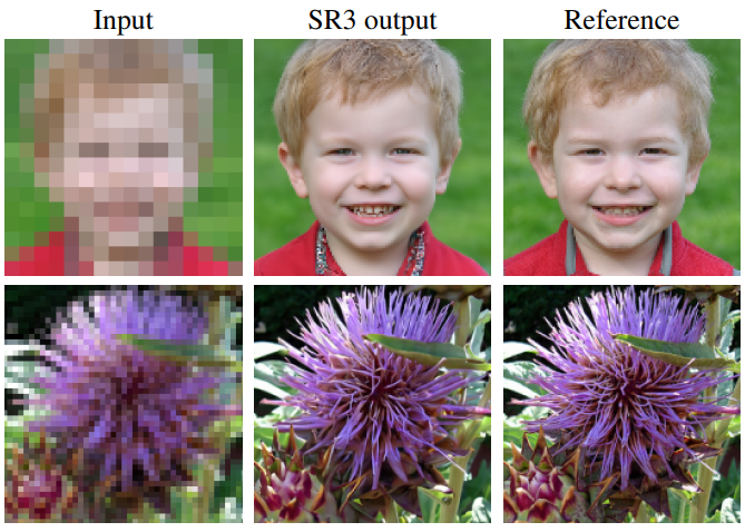
• Natural Images

다음은 ImageNet에서 학습한 SR3 Model($64 \times 64 \rightarrow 256 \times 256$)을 Test Data에 대해 평가한 것이다.

• Face Images

다음은 FFHQ에서 학습한 SR3 model($64 \times 64 \rightarrow 512 \times 512$)을 학습 셋에 포함되지 않는 이미지에서 평가한 것이다.