[Paper Review] Diffusion Models Beat GANs on Image Synthesis

이번에 리뷰할 논문은 Diffusion Model에 Condition을 주는 Classifier Guidance를 도입한 Paper이다.

해당 논문의 arXiv 링크는 다음과 같다.

Diffusion Models Beat GANs on Image Synthesis

We show that diffusion models can achieve image sample quality superior to the current state-of-the-art generative models. We achieve this on unconditional image synthesis by finding a better architecture through a series of ablations. For conditional image synthesis, we further improve sample quality with classifier guidance: a simple, compute-efficient method for trading off diversity for fidelity using gradients from a classifier. We achieve an FID of 2.97 on ImageNet 128$\times$128, 4.59 on ImageNet 256$\times$256, and 7.72 on ImageNet 512$\times$512, and we match BigGAN-deep even with as few as 25 forward passes per sample, all while maintaining better coverage of the distribution. Finally, we find that classifier guidance combines well with upsampling diffusion models, further improving FID to 3.94 on ImageNet 256$\times$256 and 3.85 on ImageNet 512$\times$512. We release our code at https://github.com/openai/guided-diffusion

arXiv.orgPrafulla Dhariwal

참고한 자료들은 다음과 같다.

Welcome to JunYoung’s blog | Improved DDPM + Diffusion beats GAN + Classifier free diffusion guidance 논문 리뷰

Improve diffusion models

Improved DDPM + Diffusion beats GAN + Classifier free diffusion guidance 논문 리뷰JunYoung

[논문리뷰] Diffusion Models Beat GANs on Image Synthesis

Diffusion Models Beat GANs on Image Synthesis 논문 리뷰

전생했더니 인공지능이었던 건에 대하여JiYeop Kim

Classifier Guidance - Diffusion Model 논문 리뷰

Classifier Guidance 논문의 핵심 내용을 리뷰합니다. 먼저 기존 방법의 문제점을 살펴봅니다. 이어서 이를 해결하기 위한 제안 방법을 살펴봅니다. 마지막으로 성능 비교 실험을 통해 Classifier Guidance의 효과를 확인합니다.

FFightingFfightingseok

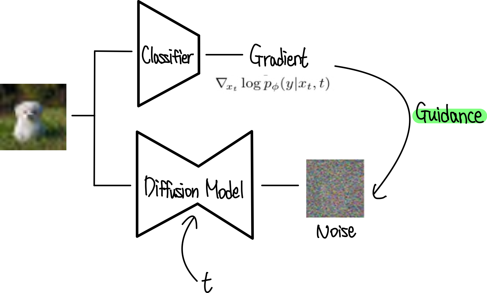
Paper Flow

해당 논문 Diffusion Models Beat GANs on Image Synthesis는 아래의 순서로 Flow가 구성되어 있다.

1) Improved DDPM

기본 Framework인 DDPM에 아래의 improvement를 적용시켜 저자들의 model에 사용한다.

• Trainable Variance: $\Sigma_\theta(x_t,t)$
• Hybrid Loss: $L_\text{hybrid} = L_\text{simple} + \lambda L_\text{vlb}$
• DDIM (Faster Sampling): $\mathbf{x}_{s} \sim q_\sigma(\mathbf{x}_{s}|\mathbf{x}_t, \mathbf{x}_0)$

2) Architecture Improvement

1. 모델 크기를 일정하게 유지하면서 depth(network 깊이) 대비 width(channel 수)증가
2. Attention head의 수 증가 (U-Net의 residual block에 attention이 들어감)
3. Attention을 $16 \times 16$ 뿐만 아니라 $32 \times 32$와 $8 \times 8$의 feature map에도 사용
4. BigGAN의 residual block을 upsampling과 downsampling에 사용
5. Residual connection을 $\frac{1}{\sqrt{2}}$로 rescale

위의 Improvement의 제안사항이 유의미한지 확인하기 위해 아래의 Ablation study를 진행한다.

- Ablation of various architecture changes


- Ablation of various attention configurations

• Adaptive Group Normalization (AdaGN)을 적용

$$\text{AdaGN}(h, y) = y_s \text{GroupNorm}(h) + y_b$$

최종적으로, 앞으로 사용하는 Final Improved Model Architecture는 다음과 같다:

• variable width with 2 residual blocks per resolution
• multiple heads with 64 channels per head
• attention @ 32, 16, 8 resolutions
• BigGAN residual blocks for up and downsampling
• AdaGAN (Adaptive Group Normalization) for injecting timestep and class embeddings into residual blocks

3) Classifier Guidance

Classifier $p_{\phi}(y|x_t, t)$을 noisy image $x_t$에서 학습시킨 뒤, 


classifier gradient $\nabla_{x_t}\log p_\phi(y|x_t, t)$를 arbitrary class label $y$ 에 대한 diffusion sampling process의 guidance로 사용한다.

• DDPM Sampler (Markovian Process): Conditional Guidance
• DDIM Sampler (Non-Markovian Process): Conditional Guidance

0. Abstract

기존의 Diffusion Model들은 ablation study를 통해 better architecture를 찾으면서 unconditional image synthesis를 수행했다.

그 결과 현재 SOTA보다 더 좋은 image sample quality를 가질 수 있었다.

반면에, Conditional Image Synthesis의 경우에는 Classifier - Guidance를 통해 sample quality를 더 향상시킬 수 있다.

이는 simple, compute-efficient method으로 classfifier gradient를 이용하여 diversity를 줄이면서 fieldity를 향상시키는 trade-off를 사용한다.

• Fieldity: Sample Quality (학습에 사용한 원본 이미지와의 유사성)
• Diversity: Sample Diversity (출력된 이미지의 분산)

이러한 Classifier - Guidance Model은 ImageNet의 $128 \times 128, 256 \times 256, 512 \times 512$에서 낮은 FID Score ($2.97, 4.59, 7.72$)를 얻었으며,

각 sample당 forward pass를 25번밖에 하지 않아도 bigGAN-deep 모델과 비슷한 성능을 내며, distribution을 더 잘 모델링한다는 장점이 있다.

저자들이 제시한 코드는 아래의 링크에서 확인할 수 있다.

GitHub - openai/guided-diffusion

Contribute to openai/guided-diffusion development by creating an account on GitHub.

GitHubopenai

1. Introduction

기존의 여러 diffusion 기반의 모델들이 놀라운 성능을 보이고 있지만, 여전히 GAN의 성능을 따라잡지는 못했으며 대부분의 데이터셋에서 state-of-the-art를 달성하지 못하였다.

하지만, 이 논문은 GAN을 제치고 대부분의 데이터셋에서 state-of-the-art가 되었다.

저자들은 diffusion model과 GAN 사이의 격차가 적어도 두 가지 요인에서 비롯된다고 가정한다.

1. 최근 GAN 논문에서 사용된 모델 아키텍처가 많이 탐구되고 정제되었다.
2. GAN은 fidelity와 diversity의 trade-off에서 fidelity를 선택하였으며, 고품질 샘플을 생성하지만 전체 분포를 포함하지는 않는다.

저자들은 먼저 모델 아키텍처를 개선한 다음 fidelity를 위해 diversity를 절충하는 방법을 고안한다. 이러한 개선 사항을 통해 여러 가지 metric과 데이터셋에서 GAN을 능가하는 새로운 모델을 만들었다.

2. Background

Background에 해당하는 Section 2에서는 Diffusion model에 대한 overview를 간단하게 다룬다. 더 자세한 수학적인 수식에 관한 설명은 아래의 포스트를 참고하자.

[Paper Review] Denoising Diffusion Probabilistic Model (DDPM)

이번에 리뷰할 논문은 DDPM이라 불리는 Denoising Diffusion Probabilistic Model이다. 해당 Paper는 아래의 링크에서 찾을 수 있다. Denoising Diffusion Probabilistic ModelsWe present high quality image synthesis results using diffusion probabilistic models, a class of latent variable models inspired by considerations from nonequilibrium thermodynamics. Our best results are obtained by training on

Action Precedes MotivationJaewon Kim

Diffusion Model들은 gradual Forward Process(noising, diffusion)를 reverse시킨 Reverse Process(denoising, sampling)의 distribution에서 sample을 modeling한다.

구체적으로, Reverse Process는 noise $x_T$에서 denoising 과정을 통해 less-noisy sample $x_{T-1}, x_{T-2}, \cdots, x_0$을 얻는 과정이다.

• noise: $x_T$
• signal: $x_0$
• noisy sample(image): $x_t$

매 time step $t$마다 특정 noise level에 대응되며, $x_t$는 signal $x_0$와 gaussian noise $\epsilon$의 결합으로 구성되어 있다.

이때, Noise scheduling에 대한 SNR (Signal-to-Noise Ratio)는 time step $t$에 의해 결정된다.


Natural Image에 잘 작용되고, various derivation을 간소화시킬 수 있기에, Noise $\epsilon$은 $\epsilon \sim \mathcal{N}(0, \mathbf{I})$ Diagnal Gaussian Distribution으로부터 sampling 되었다고 가정한다.

Diffusion model은 $x_t$로부터 noise가 덜 있는 $x_{t-1}$을 생성하도록 학습된다. DDPM 논문에서는 모델을 함수 $\epsilon_\theta(x_t,t)$로 parameterize하여 $x_t$의 gaussian noise 부분을 예측하도록 하였다.

이 모델을 학습시키기 위해서는 데이터(signal) $x_0$, timestep $t$, noise $\epsilon \sim \mathcal{N}(0,I)$로 관련하게 만들어진 샘플 $x_t$가 minibatch에 포함되어야 한다.

학습에 사용하는 training objectve (loss function)는 $|\epsilon_\theta(x_t,t) - \epsilon|^2$이고, 실제 noise $\epsilon$과 예측된 noise $\epsilon_\theta$의 간단한 mean-squared error loss를 구성한다.

DDPM에서는 reasonable assumption을 통해, Reverse Process $p_\theta(x_{t-1}|x_t)$를 Diagonal Gaussian Distribution $\mathcal{N}(x_{t-1}; \mu_\theta(x_t,t), \Sigma_\theta(x_t,t))$으로 modeling할 수 있다고 한다.

• Mean: $\mu_\theta(x_t,t)$는 $\epsilon_\theta(x_t,t)$로부터 계산가능

$$\mu_\theta(x_t,t) = \frac{1}{\sqrt{\alpha}_t}\left(\mathbf{x}_t(\mathbf{x}_0,\epsilon) - \frac{\beta_t}{\sqrt{1-\bar{\alpha}_t}}\epsilon_{\theta}(\mathbf{x}_t, t)\right)$$

• Variance: $\Sigma_\theta(x_t,t)$는 상수 $\tilde{\beta}_t \: \text{or} \beta_t$라는 time-dependent constant로 놓거나 separate neural network head로 설정하여 학습가능하도록 놓을 수 있다.

또한, 실제 variational lower bound $L_\text{vlb}$보다 간단한 mean-squared error 목적 함수 $L_\text{simple}$이 더 좋은 결과를 나타낸다.

$$L_{\text{vlb}} = \mathbb{E}_{q(\mathbf{x}_{0:T})}\left[D_{KL}(q(\mathbf{x}_T | \mathbf{x}_0)||p(\mathbf{x}_T)) + \sum_{t=2}^T D_{KL}(q(\mathbf{x}_{t-1} | \mathbf{x}_t, \mathbf{x}_0)||p_\theta(\mathbf{x}_{t-1} |\mathbf{x}_t)) -\log p_\theta(\mathbf{x}_0 | \mathbf{x}_1)\right]$$


$$L_{\text{simple}}=\mathbb{E}_{\mathbf{x}_0,\epsilon} \left[ ||\epsilon - \epsilon_\theta(\sqrt{\bar{\alpha_t}}\mathbf{x}_0 + \sqrt{1 - \bar{\alpha_t}}\epsilon, t)||^2 \right]$$

뿐만 아니라, 이 Training Objective를 이용하여 training시키고, 이에 대응되는 sampling procedure를 사용하는 것은 Denoising Score Matching Model을 사용하는 것과 동일하다고 한다.

• 위의 Model은 Langevin dynamics를 이용하여 multiple noise level을 이용하여 train된 denoising model에서 sampling을 시도한다.

2.1) Improvements

Section 2.1부분에서는 해당 논문에 저자들이 채용한 Proposed Improvements to diffusion models 들을 소개한다.

크게 3가지인데, 저자들이 기본적으로 사용하는 DDPM framework에서 trainable variance, hybrid loss와 faster sampling을 위해 아래의 사항들을 메인으로 한다.

• Improved DDPM: Trainable Variance, Hybrid loss
• DDIM: Faster Sampling

Improved DDPM 논문에서도 faster sampling할 수는 있었으나, 이는 training process 자체를 바꿨기에, 모든 time step $t$에서 DDPM동일한 Marginal $q_\sigma(\mathbf{x}_{t}|\mathbf{x}_0)$를 가지도록 Non-Markovian Posterior $q_\sigma(\mathbf{x}_{t-1}|\mathbf{x}_t, \mathbf{x}_0)$를 모델링하는 DDIM과는 다르다.


즉, 'Training Process'를 바꿨는가와 'Sampling Process'를 바꿨는지로 차이가 나뉜다.

Improved DDPM 논문은 분산 $\Sigma_\theta(x_t,t)$를 상수로 고정하는 것이 차선책이며, 다음과 같이 $\Sigma_\theta(x_t,t)$를 trainable하도록 parameterize하는 것을 제안하였다.

$$\Sigma_\theta(x_t,t) = \exp(v \log \beta_t + (1-v) \log \tilde{\beta}_t) = (\beta_t)^v(\tilde{\beta_t})^{1-v}$$

$$\sigma_t^{2} = \beta_t \: \text{or} \: \sigma_t^{2} = \tilde{\beta_t}$$


$$\tilde{\beta}_t := \frac{1-\bar{\alpha}_{t-1}}{1-\bar{\alpha}_t}\beta_t$$

$v$를 출력하는 모델을 두어 Reverse Process의 variance인 upper bound $\beta_t$와 lower bound$ \tilde{\beta}_t$ 사이로 interpolate한다.

또한 위와 같이 trainable variance를 사용할 경우, $\epsilon_\theta(x_t,t)$와 $\Sigma_\theta(x_t,t)$를 모두 학습하기 위하여 Hybrid Loss $L_\text{simple} + \lambda L_\text{vlb}$를 목적 함수로 사용한다. ($\lambda = 0.001$)

$$L_\text{hybrid} = L_\text{simple} + \lambda L_\text{vlb}$$

위와 같이 Hybrid Loss를 사용할 경우, Reverse process에서의 variance를 학습할 수 있으며 이는 sample quality를 어느정도 유지하면서 더 적은 step으로 sampling을 할 수 있도록 한다.

DDIM 논문은 모든 time step $t$에서 DDPM과 같은 forward marginals $q_\sigma(\mathbf{x}_{t}|\mathbf{x}_0)$ 를 가지지만, reverse noise의 분산을 변경하여 다른 reverse sampling이 가능한 non-Markovian noising process Posterior $q_\sigma(\mathbf{x}_{t-1}|\mathbf{x}_t, \mathbf{x}_0)$를 모델링을 제안하였다.

DDPM과 동일한 training objective (forward marginal) 이지만, 서로 다른 Sampling Process due to Non-Markovian forward posterior.

Noise를 0으로 두면 $\epsilon_\theta$가 deterministic하게 latent와 이미지를 mapping하게 되어 더 적은 step으로 샘플링이 가능하다.

2.2) Sample Quality Metrics

Model들이 생성하는 Sample Quality를 비교하기 위해, 저자들은 Quantitative Evaluations들에 해당하는 Metric을 사용한다.

위의 metric들은 실제 상황에서도 사용되거나, 인간의 판단과 잘 일치하는 경우가 많지만 완벽하지 않으며 sample quality evaluation을 위해 더 좋은 metric을 찾는 것은 아직도 open problem이다.

Inception Score는 Model이 얼마나 잘 전체 ImageNet class distribution을 잘 모델링하고 있는지와, 생성된 individual sample이 하나의 class에서 생성된 것과 같이 보이는지를 평가한다.

$$IS(G) = exp(\mathbb{E}_{x\sim G}(D_{KL}(p(y|x) \parallel p(y))))$$

• $p(y)$: 실제로 생성되는 sample들이 전체 class에 대해 고르게 잘 만들어지는지를 측정
• $p(y|x)$: 생성된 sample의 quality

1) 전체 Class의 Distribution


2) 각 Class안의 Sample Quality

다만, Inception Score는 하나의 class안에서의 distribution을 모델링하거나, diversity를 평가하지 못하기에 만약 어떠한 model이 전체 dataset의 small subset만을 기억하고 있어도 그 quality가 높다면 IS가 높을 수 있다.

즉, 각 class별로 다양한 이미지를 생성하지 못하는 경우 IS가 반영하지 못한다.


예를 들어, CIFAR-10 Dataset에 대해 10개의 class 각각에 대해 모두 quality가 높은 한 가지의 sample만 생성해내더라도, IS상으로는 높은 결과가 나온다.


이는 Collapse를 판별할 수 없게 되는 것이다.

FID는 위의 IS의 단점을 극복하기 위해 Inception Network에서의 Layer Feature를 사용하고, Expectation 및 Covariance를 사용하여 Multivariate Gaussian Distribution을 모델링하는 방식이다.

이는 Inception-V3 latent space에 있는 두 image distribution의 distance에 대한 symmetric measure이다.

$$FID(x, g) = | \mu_x - \mu_g |_2^2 + Tr(\Sigma_x + \Sigma_g - 2(\Sigma_x\Sigma_g)^{1/2})$$

최근에는 FID의 새로운 버젼이 제시됐는데, standard pool feature 보다는 spatial feature들을 사용하는 것이다.

이렇게 할 경우, 해당 metric이 spatial feature를 더 잘 capture할 수 있으며, coherent high-level structure으로 image distribution을 모델링할 수 있다.

기존보다 개선된 Precision과 Recall을 Metric으로 사용하는 방법이 제안되었다. 이를 Metric으로 이용하여 sample fieldity와 diversity를 평가할 수 있다.

• Precision: generated sample들 중에 real sample distribution안에 들어가는 비율 (sample fieldity)
  • generated sample이 분모에 들어가므로, 내가 생성한 sample들이 모두 real sample distribution으로 mapping될 수록 sample의 quality가 올라가기에, precision은 sample fieldity와 관련

• Recall: real sample들 중에 generated sample distribution안에 들어가는 비율 (sample diversity)
  • real sample이 분모에 들어가므로, 실제 sample의 class들을 반영하는 생성된 sample이 많을수록 diversity가 올라가기에, recall은 sample distribution과 관련

아래의 그림을 보면, 모델이 학습한 implicit probability가 $P_g$이고, 실제 sample distribution이 $P_r$이라 하자.

• $\text{TP}$: $P_g$에 해당되는 sample이면서 $P_r$에 포함되는 것
• $\text{FP}$: $P_g$에 해당되는 sample이면서 $P_r$에 포함되지 않는 것
• $\text{FN}$: $P_g$에 해당되지 않는 sample이면서 $P_r$에 포함된 것

$$\text{Precision} = \frac {TP} {TP + FP} $$

- Sampling Fieldity (Quality)

$$\text{Recall} = \frac {TP} {TP + FN} $$

- Sampling Diversity

저자들은 FID를 default metric으로 사용하여 전반적인 sample quality를 비교했다.

FID는 sample diversity와 fieldity 모두를 capture할 수 있기에 SOTA를 평가하는데 있어 standard metric이 될 수 있다.

• sample diversity & fieldity: FID
• sample diversity (distribution coverage): Recall
• sample fieldity: Precision and IS

일관적인 비교를 위해, entire training set을 reference batch로 사용하고, 모든 모델들에 대한 evaluation metric들은 동일한 codebase를 사용한다.

3. Architectural Improvements

Section 3인 Architectural Improvements는 several architecture에 대해 ablation study를 수행하며 best sample quality를 제공하는 diffusion model의 최적 architecture를 찾는다.

DDPM은 U-Net Architecture를 사용한다.

U-Net은 residual layer와 downsampling/upsampling convolution을 쌓아 구성하며 크기가 같은 layer끼리 skip connection으로 연결한다.

추가로, $16 \times 16$ feature map에는 single-head global attention을 사용하였으며, 각 residual block에 timestep embedding의 projection을 넣어주었다.

저자들은 다음의 Architectural Change를 통해 much larger and more diverse한 dataset에서의 더 높은 resolution의 sample quality를 높일 수 있음을 보였다.

1. 모델 크기를 일정하게 유지하면서 depth(network 깊이) 대비 width(channel 수)증가
2. Attention head의 수 증가 (U-Net의 residual block에 attention이 들어감)
3. Attention을 $16 \times 16$ 뿐만 아니라 $32 \times 32$와 $8 \times 8$의 feature map에도 사용
4. BigGAN의 residual block을 upsampling과 downsampling에 사용
5. Residual connection을 $\frac{1}{\sqrt{2}}$로 rescale

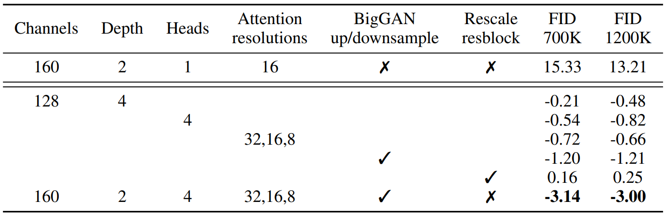
Section 3에 있는 모든 Comparison들은 ImageNet $128 \times 128$에서 batch size 256, sampling step 250으로 고정하고 학습한 모델의 FID는 아래 표와 같다.

표를 해석할 때, 위에서 아래로 갈 수록 앞에서 언급한 5개의 Architectural Change를 greedy하게 누적해서 적용하고 있는 것으로 보자.


그렇기에 FID score가 change가 누적해서 작용하기에 계속해서 감소하다가 Residual Block Rescale에 올 때 다시 증가한다.


이는 Rescaling이 실제로 성능을 개선시키지 못하는 것으로 해석가능하다.

Residual connection을 rescale하는 것을 제외하고는 모두 성능이 개선되었으며 4개의 Architectural Change들을 같이 사용하였을 때 긍정적인 효과를 보였다.

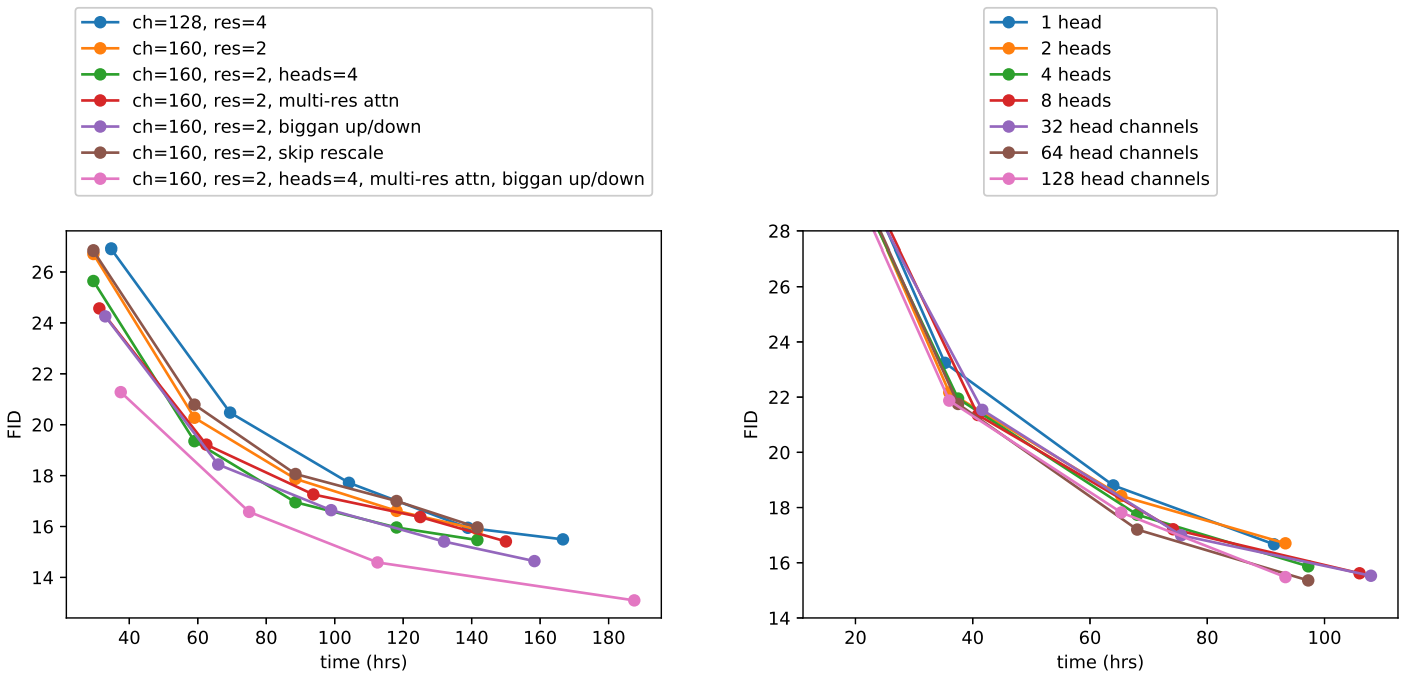
다만, 위 그래프에서 볼 수 있듯이 depth가 증가하면 성능에 도움이 되지만 training time이 늘어나고 wider model과 동일한 성능에 도달하는 데 시간이 더 오래 걸리므로 추가 실험에서 이 변경 사항을 사용하지 않기로 결정했다고 한다.

또한 저자들은 Transformer architecture와 더 잘 일치하는 다른 attention 구성을 연구하였다.

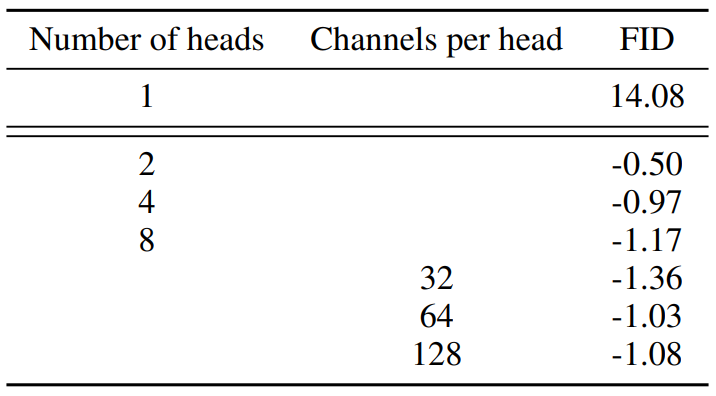
이를 위해 number of attention head를 constant로 고정하거나 number of channels per head를 고정하는 실험을 했다.

나머지 아키텍처에서는 128 base channels, resolution당 2개의 residual block, multi-resolution attention, BigGAN up/downsampling을 사용하고 700k iteration에 대해 모델을 학습한다.

위의 Table의 결과는 아래의 사항들을 보여준다:

• more heads
• fewer channels per head

다른 하나가 고정된 채, 나머지가 일어나면 FID는 감소한다. (Improvement)

위 그래프에서 64 channels이 wall-clock time에 가장 적합하다는 것을 알 수 있다.

따라서 64 channels per head을 기본값으로 사용한다.

저자들은 이 선택이 modern transformer architecture와 더 잘 일치하고 다른 구성과 동등하다는 점에 주목하였다.

3.1) Adaptive Group Normalization

저자들은 Adaptive Group Normalization(AdaGN)이라는 layer로도 실험을 진행하였다.

이 layer는 hidden layer activation $h$에 group normalization 적용 후 각 residual block에 timestep embedding과 class embedding을 AdaIN이나 FiLM과 같은 방법으로 결합한다.

$$\text{AdaGN}(h, y) = y_s \text{GroupNorm}(h) + y_b$$

• $h$: intermediate activations(hidden layer activation) of the residual block
• $y = [y_s, y_b]$: linear projection of timestep embedding and class embedding

AdaGN이 좋은 성능을 보였기에 모든 Diffusion Model에 적용하여 improvement를 이뤘으나, 특별히 Ablation Study를 진행한 결과는 다음과 같다.

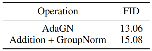
위 Table 에서 AdaGN이 실제로 FID를 개선하는 것을 볼 수 있다.

위의 두 모델은 다음의 spec을 고정한채 사용한다.


128 base channels, 2 residual blocks per resolution, multi-resolution attention with 64 channels per head, BigGAN up/down sampling, trained for 700k iterations.

최종적으로, 앞으로 사용하는 Final Improved Model Architecture는 다음과 같다:

• variable width with 2 residual blocks per resolution
• multiple heads with 64 channels per head
• attention @ 32, 16, 8 resolutions
• BigGAN residual blocks for up and downsampling
• AdaGAN (Adaptive Group Normalization) for injecting timestep and class embeddings into residual blocks

4. Classifier Guidance

well-designed architecture를 사용하는 것 외에도 conditional image synthesis을 위한 GAN은 class label을 많이 사용한다.

GAN에서 Class label을 사용하는 방법은 다음과 같다:

• 1) classifier $p(y|x)$처럼 동작하도록 설계된 head가 있는 Discriminator를 사용
• 2) class-conditional normalization 방법을 사용

이전 논문에서는 label-limited rigme에서 synthetic label을생성하는 것이 도움이 된다는 것을 발견했으며, 이는 클래스 정보가 중요하다는 것을 의미한다.

GAN에서의 이러한 연구들을 생각했을 때 class label들을 diffusion model에 conditioning하는 다양한 방법이 필요하다.

현재 이미 위에서 class embedding과 time step embeddin을 일종의 style 정보로 AdaGN(Adaptive GroupNorm)을 통해 주입하고 있다.

하지만, class embedding을 넣어주는 과정은 실제로 discriminator 정보를 explicit하게 주는 것과는 차이가 있다.

여기에서 diffusion generator를 개선하기 위해 classifier $p(y|x)$를 활용하는 다른 접근 방식이 필요하다.

Sohl-Dickstein et al.와 Song et al.은 classifier gradient를 사용하여 pre-trained diffusion model을 conditioning한다.

Score-Based Generative Modeling through Stochastic Differential Equations

Creating noise from data is easy; creating data from noise is generative modeling. We present a stochastic differential equation (SDE) that smoothly transforms a complex data distribution to a known prior distribution by slowly injecting noise, and a corresponding reverse-time SDE that transforms the prior distribution back into the data distribution by slowly removing the noise. Crucially, the reverse-time SDE depends only on the time-dependent gradient field (\aka, score) of the perturbed data distribution. By leveraging advances in score-based generative modeling, we can accurately estimate these scores with neural networks, and use numerical SDE solvers to generate samples. We show that this framework encapsulates previous approaches in score-based generative modeling and diffusion probabilistic modeling, allowing for new sampling procedures and new modeling capabilities. In particular, we introduce a predictor-corrector framework to correct errors in the evolution of the discretized reverse-time SDE. We also derive an equivalent neural ODE that samples from the same distribution as the SDE, but additionally enables exact likelihood computation, and improved sampling efficiency. In addition, we provide a new way to solve inverse problems with score-based models, as demonstrated with experiments on class-conditional generation, image inpainting, and colorization. Combined with multiple architectural improvements, we achieve record-breaking performance for unconditional image generation on CIFAR-10 with an Inception score of 9.89 and FID of 2.20, a competitive likelihood of 2.99 bits/dim, and demonstrate high fidelity generation of 1024 x 1024 images for the first time from a score-based generative model.

arXiv.orgYang Song

Deep Unsupervised Learning using Nonequilibrium Thermodynamics

A central problem in machine learning involves modeling complex data-sets using highly flexible families of probability distributions in which learning, sampling, inference, and evaluation are still analytically or computationally tractable. Here, we develop an approach that simultaneously achieves both flexibility and tractability. The essential idea, inspired by non-equilibrium statistical physics, is to systematically and slowly destroy structure in a data distribution through an iterative forward diffusion process. We then learn a reverse diffusion process that restores structure in data, yielding a highly flexible and tractable generative model of the data. This approach allows us to rapidly learn, sample from, and evaluate probabilities in deep generative models with thousands of layers or time steps, as well as to compute conditional and posterior probabilities under the learned model. We additionally release an open source reference implementation of the algorithm.

arXiv.orgJascha Sohl-Dickstein

Classifier $p_{\phi}(y|x_t, t)$을 noisy image $x_t$에서 학습시킨 뒤, 


classifier gradient $\nabla_{x_t}\log p_\phi(y|x_t, t)$를 arbitrary class label $y$ 로 diffusion sampling process를 guide하는데 사용한다.

• noise: $x_T$
• signal: $x_0$
• noisy sample(image): $x_t$
• arbitrary class label: $y$
• Classifier: $p_{\phi}(y|x_t, t)$
• classifier gradient: $\nabla_{x_t}\log p_\phi(y|x_t, t)$

Section 4는 크게 2가지의 Section으로 구분되어 있는데, Section 4.1, 4.2에서는 classifier를 사용하여 conditional sampling processes를 유도하는 두 가지 방법을 설명한다.

• DDPM Sampler (Markovian Process): Conditional Guidance
• DDIM Sampler (Non-Markovian Process): Conditional Guidance

이후 Section 4.3에서는 이러한 classifier를 실제로 사용하여 샘플 품질을 개선하는 방법을 설명한다.

간결함을 위해 $p_{\phi}(y|x_t, t) = p_{\phi}(y|x_t)$와 $\epsilon_\theta(x_t, t) = \epsilon_\theta(x_t)$를 사용한다.

4.1) Conditional Reverse Noising Process

Unconditional reverse denoising process가 $p_\theta(x_t|x_{t+1})$인 diffusion model을 label $y$로 conditioning 다음과 같이 생성한다는 것으로 출발한다.

Conditional Reverse Denoising Process = Conditional Sampling Process는 다음과 같이 모델링된다.

$$p_{\theta,\phi}(x_t|x_{t+1},y) = Zp_\theta(x_t|x_{t+1})p_\phi(y|x_t)$$

• Pre-trained Classifier: $p_\phi(y|x_t)$
• Unconditional Reverse Process: $p_\theta(x_t|x_{t+1})$

위의 pre-trained classifier는 diffusion process에 대해 완전히 explicit한 정보이기에 normalizing factor $Z$에 대해 constant 취급이 가능하다.

$Z$는 합을 분모의 합을 1로 만들기 위한 normalizing factor이다.

일반적으로 reverse process는 intractable하기에 distribution에서 바로 sampling을 할 수 없지만, Sohl-Dickstein et al.은 이 분포를 perturbed Gaussian distribution으로 근사할 수 있음을 보였다.

Diffusion model이 time step $x_{t+1}$가 주어졌을 때 previous timestep $x_t$의 분포를 Gaussian Distribution을 사용해서 예측하기 때문에 다음과 같다.

즉, Unconditional Reverse Process $p_\theta(x_t|x_{t+1})$는 다음과 같이 log-likelihood로 표현가능하다. (Multivariate gaussian)

$$p_\theta(x_t|x_{t+1}) = \mathcal{N}(\mu, \Sigma)$$


$$\log p_\theta(x_t|x_{t+1}) = -\frac{1}{2}(x_t - \mu)^T \Sigma^{-1} (x_t - \mu) + C$$

$\log p_\phi(y|x_t)$가 $\Sigma^{-1}$보다 낮은 곡률을 가진다고 가정할 수 있다. 이 가정은 diffusion step의 수가 무한에 가까워질 때 $|\Sigma| \to 0$이 되어 합리적이게 된다.

• $p_{\theta,\phi}(x_t|x_{t+1},y) = Zp_\theta(x_t|x_{t+1})p_\phi(y|x_t)$
• $\log p_\theta(x_t|x_{t+1}) = -\frac{1}{2}(x_t - \mu)^T \Sigma^{-1} (x_t - \mu) + C$

$\log p_\theta(x_t|x_{t+1})$는 $-\frac{1} {2}\Sigma^{-1}$를 계수로 갖는 Quadratic function이다.


$\Sigma^{-1}$는 아래의 식에 의해 $||\Sigma||$를 분모로 가지므로 $||\Sigma|| \rightarrow 0$이 될 때 매우 커지게 되어 결과적으로 Quadratic function의 곡률(계수)가 커지게 된다.

따라서, classifier $p_\phi$가 가지는 곡률이 unconditional reverse process인 $p_\theta$보다 더 작을 것이라고 가정할 수 있는 것이다.

이 경우, $x_t = \mu$ 근처에서 Taylor Series 1차 전개를 사용하여 Classifier Guidance 부분인 $\log p_\phi(y|x_t)$를 근사할 수 있다:

즉, 어차피 sampling 되는 part는 $\mu$가 메인인데 $x_t = \mu$인 point에서 $p_\theta$ 대비 $p_\phi$가 가지는 곡률이 상대적으로 매우 작기에 무시가능하다는 것이다.

$$\log p_\phi(y|x_t) \approx \log p_\phi(y|x_t)|_{x_t=\mu} + (x_t - \mu)\nabla{x_t} \log p_\phi(y|x_t)|_{x_t=\mu}$$ $$= (x_t - \mu)g + C_1$$

여기서 $g = \nabla_{x_t} \log p_\phi(y|x_t)|_{x_t=\mu}$이고 $C_1$은 상수이다.

이를 대입하면 다음과 같다.

$$\log(p_\theta(x_t|x_{t+1})p_\phi(y|x_t)) = \log(p_\theta(x_t|x_{t+1})) + \log(p_\phi(y|x_t)) $$

$$\approx -\frac{1}{2}(x_t - \mu)^T \Sigma^{-1} (x_t - \mu) + (x_t - \mu)g + C_2$$

$$= -\frac{1}{2}(x_t - \mu - \Sigma g)^T \Sigma^{-1} (x_t - \mu - \Sigma g) + \frac{1}{2}g^T\Sigma g + C_2$$

$$= -\frac{1}{2}(x_t - \mu - \Sigma g)^T \Sigma^{-1} (x_t - \mu - \Sigma g) + C_3$$

$$= \log p(z) + C_4, \quad z \sim \mathcal{N}(\mu + \Sigma g, \Sigma)$$

$C_4$는 정규화 상수 $Z$에 해당하기 때문에 무시할 수 있다.

따라서 conditional transition operator를 unconditional transition operator와 유사한 가우시안 분포로 근사할 수 있으며, 이 때 평균이 $\Sigma g$만큼 이동한다.

Algorithm 1은 Classifier guided diffusion sampling(DDPM)을 보여준다.

뒤의 섹션에서 기울기에 대한 scale factor $s$를 포함하며 자세히 설명한다.

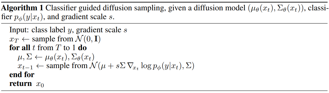
결국 Classifier Guidance에 의한 conditional sampling process(DDPM Sampler)는 pre-trained classifier gradient를 이용하여 $\mu$를 shift시킨다고 볼 수 있다.

4.2) Conditional Sampling for DDIM

위의 conditional sampling process에 대한 derivation는 stochastic diffusion sampling에만 유효하며 DDIM과 같은 deterministic sampling process에는 적용할 수 없다.

이를 위해 아래의 논문에서 사용한 diffusion model과 score matching 사이의 연결을 활용하는 score-based conditioning trick을 사용한다.

Score-Based Generative Modeling through Stochastic Differential Equations

Creating noise from data is easy; creating data from noise is generative modeling. We present a stochastic differential equation (SDE) that smoothly transforms a complex data distribution to a known prior distribution by slowly injecting noise, and a corresponding reverse-time SDE that transforms the prior distribution back into the data distribution by slowly removing the noise. Crucially, the reverse-time SDE depends only on the time-dependent gradient field (\aka, score) of the perturbed data distribution. By leveraging advances in score-based generative modeling, we can accurately estimate these scores with neural networks, and use numerical SDE solvers to generate samples. We show that this framework encapsulates previous approaches in score-based generative modeling and diffusion probabilistic modeling, allowing for new sampling procedures and new modeling capabilities. In particular, we introduce a predictor-corrector framework to correct errors in the evolution of the discretized reverse-time SDE. We also derive an equivalent neural ODE that samples from the same distribution as the SDE, but additionally enables exact likelihood computation, and improved sampling efficiency. In addition, we provide a new way to solve inverse problems with score-based models, as demonstrated with experiments on class-conditional generation, image inpainting, and colorization. Combined with multiple architectural improvements, we achieve record-breaking performance for unconditional image generation on CIFAR-10 with an Inception score of 9.89 and FID of 2.20, a competitive likelihood of 2.99 bits/dim, and demonstrate high fidelity generation of 1024 x 1024 images for the first time from a score-based generative model.

arXiv.orgYang Song

특히 샘플에 추가된 noise를 예측하는 모델 $\epsilon_\theta(x_t)$가 있는 경우 다음과 같이 score function을 도출하는 데 사용할 수 있다.

$$\nabla_{x_t} \log p_\theta(x_t) = -\frac{1}{\sqrt{1-\bar{\alpha}t}}\epsilon_\theta(x_t)$$

위 식을 $p(x_t)p(y|x_t)$의 score function에 대입하면 다음과 같다.

$$\nabla_{x_t} \log(p_\theta(x_t)p_\phi(y|x_t)) = \nabla_{x_t} \log p_\theta(x_t) + \nabla_{x_t} \log p_\phi(y|x_t)$$

$$= -\frac{1}{\sqrt{1-\bar{\alpha}_t}}\epsilon_\theta(x_t) + \nabla_{x_t} \log p_\phi(y|x_t) = -\frac{1}{\sqrt{1-\bar{\alpha}_t}}\hat{\epsilon}(x_t)$$

결과 분포에 대응되는 새로운 epsilon 예측 $\hat{\epsilon}(x_t)$을 다음과 같이 정의할 수 있다.

$$\hat{\epsilon}(x_t) := \epsilon_\theta(x_t) - \sqrt{1-\bar{\alpha}_t}\nabla_{x_t} \log p_\phi(y|x_t)$$

$\epsilon_\theta(x_t)$ 대신 $\hat{\epsilon}(x_t)$을 사용하면 DDIM에서 사용하는 샘플링 과정을 사용할 수 있다. 이 샘플링 과정은 Algorithm 2와 같다.

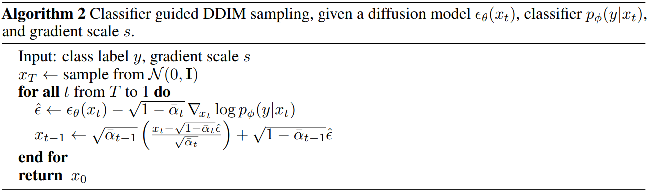
결국 Classifier Guidance에 의한 conditional sampling process(DDIM Sampler)는 pre-trained classifier gradient를 이용하여 noise $\epsilon$를 shift시키고, 해당 noise를 이용하여 sampling하는 것을 볼 수 있다.

4.3) Scaling Classifier Gradients

Classifier $p_\phi$가 class guidance를 주기 위해서는 Classification model이 학습되어야 한다.

즉, 저자들은 large-scale generative task에 classifier guidance를 적용하기 위해 ImageNet에서 classification model을 학습시켰다.

Classifier의 아키텍처는 최종 출력을 생성하기 위해 $8 \times 8$ layer에 attention pool이 있는 UNet 모델의 downsampling 부분을 사용하였다.

해당 diffusion model과 동일한 noising 분포에서 이러한 classifier를 학습시키고 과적합을 줄이기 위해 random crop을 추가하였다.

Classifier는 각 noise step에 대해 분류할 수 있어야 하므로, 각각의 time step에 대한 noised input을 학습하게 된다.


학습 이후에는 pre-trained classifier를 이용하여 classifier gradient를 사용해 conditional sampling을 진행하게 된다.

학습 후 Algorithm 1에 설명된 대로 classifier를 diffusion model의 샘플링 프로세스에 통합하였다.

저자들은 unconditional ImageNet 모델을 사용한 초기 실험에서는 classifier gradient를 1보다 큰 상수로 scaling해야 한다는 것을 발견했다.

unconditional ImageNet 모델은 class condition을 따로 embedding으로 주지 않은 Network를 의미한다.

Scale로 1을 사용하면 classifier가 합리적인 확률(약 50%)을 원하는 클래스에 할당한다.

그러나 실제로 확인해보면 이러한 샘플들은 의도한 클래스와 일치하지 않는다.

Classifier gradient를 scaling하면 이 문제가 해결되었고 classifier의 클래스 확률이 거의 100%로 증가한다.

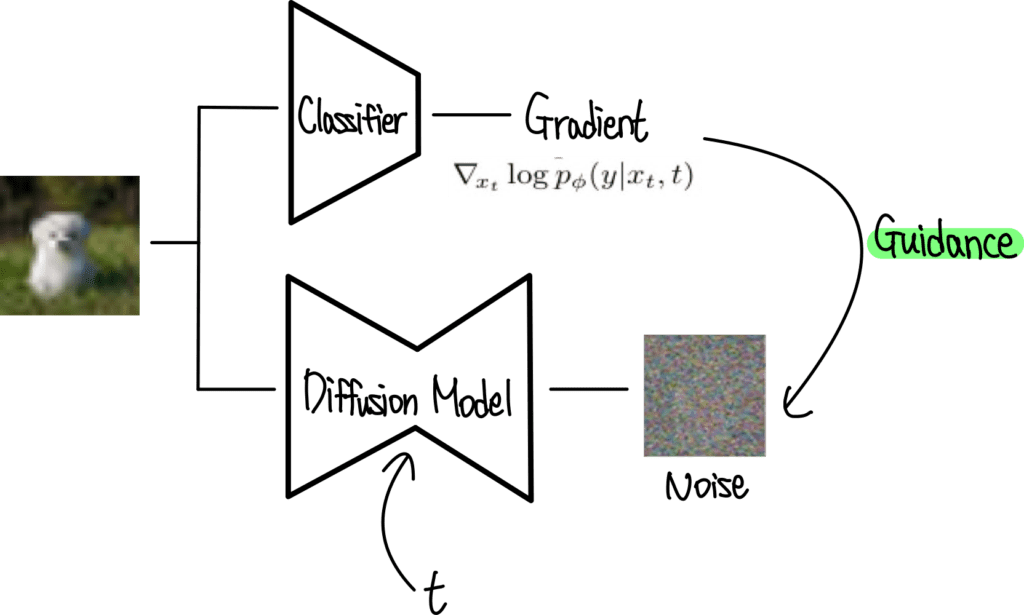
아래 그림은 이 효과의 예를 보여준다.

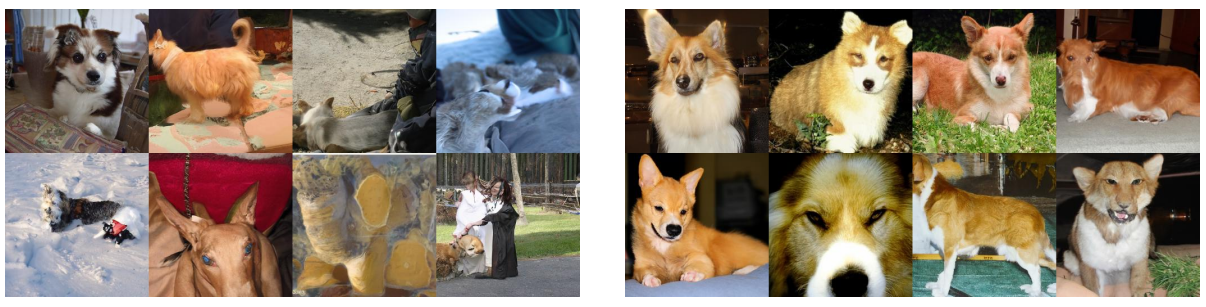
위 그림은 classifier guidance를 사용한 unconditional diffusion model에 "Pembroke Welsh corgi"를 condition으로 주고 샘플링한 결과이다.

왼쪽은 classifier scale로 1.0을 사용하였고 오른쪽은 10.0을 사용하였다. FID는 왼쪽이 33.0, 오른쪽이 12.0으로 클래스에 더 일치하는 이미지가 생성되었다.

Scaling classifier gradient의 효과는

$$s \cdot \nabla_x \log p(y|x) = \nabla_x \log \frac{1}{Z}p(y|x)^s$$

로부터 이해할 수 있다. ($Z$는 정규화 상수)

결과적으로 conditioning process는 $p(y|x)^s$에 비례하는 re-normalized classifier distribution에 근거한다.

$s > 1$일 때 지수에 의해 값이 증폭되기 때문에 $p(y|x)^s \approx p(y|x)$보다 더 뾰족해진다.

즉, 더 큰 scale $s$를 사용하면 classifier의 mode들에 더 조밀해 맞추며, 이는 더 높은 fidelity의 (그러나 더 낮은 diversity의) 샘플을 생성하는 데 잠재적으로 바람직하다.

위의 실험에서 기본 diffusion model이 $p(x)$를 모델링하고 unconditional이라고 가정했다.

그러나, 정확히 동일한 방식으로 conditional diffusion model $p(x|y)$를 학습시키고 classifier guidance를 사용할 수 있다.

아래 표는 unconditional model과 conditional model 모두의 샘플 품질이 classifier guidance에 의해 크게 향상될 수 있음을 보여준다.

• conditional model: $p(y|x)$ Modeling
• unconditional model: $p(x)$ Modeling

Conditional Model은 위의 AdaGN(Adaptive GroupNorm)를 사용하여 class embedding과 timestep embedding을 같이 residual block에 반영하는 conditional diffusion이고,


Unconditional Model은 AdaGN, concat 등으로 class label을 사용하지 않고, timestep embedding만 반영하는 conditional diffusion을 의미한다.

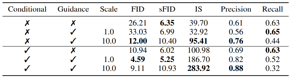
(ImageNet 256×256를 배치 사이즈 256으로 200만 iteration동안 학습)

클래스 레이블을 사용하여 직접 학습시키는 것이 여전히 도움이 되지만 중요한 높은 scale로 guide된 unconditional model이 guide되지 않은 conditional model의 FID에 상당히 근접할 수 있음을 알 수 있다.

물론 conditional model을 guide하면 FID가 더욱 좋아된다.

또한 classifier guidance가 recall을 희생시키고 precision을 향상시켜 샘플의 fidelity와 diversity 사이의 trade-off를 도입함을 보여준다.

아래 그래프에서 gradient scale에 따라 이 trade-off가 어떻게 달라지는지 볼 수 있다.

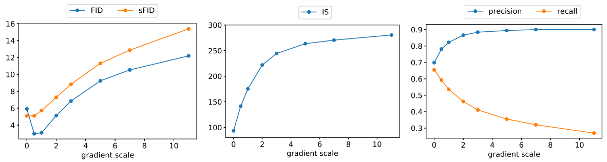
1.0 이상의 scale을 사용하면 recall (diversity의 척도)을 더 높은 precision과 IS (fidelity의 척도)로 잘 교환된다.

FID와 sFID는 fidelity와 diversity 모두에 의존하기 때문에 중간 지점에서 최상의 값을 얻는다.

또한 아래 그림에서 BigGAN의 truncation trick과 classifier guidance를 비교한다.

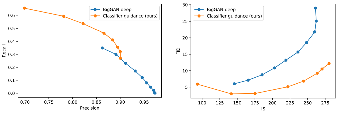
FID를 IS로 절충할 때 classifier guidance가 BigGAN-deep보다 훨씬 낫다는 것을 알 수 있다.

Precision/recall trade-off 그래프는 classifier guidance가 특정 precision 값까지만 더 나은 선택이며 그 이후에는 더 나은 precision을 달성할 수 없음을 보여준다.

5. Results

5.1) State-of-art Image Synthesis

저자들은 unconditional image generation의 평가를 위해 LSUN의 bedroom, horse, cat 데이터셋에서 학습을 진행하였다.

Classifier guidance의 평가를 위해 ImageNet의 $128 \times 128, 256 \times 256, 512 \times 512$ 크기에 대하여 conditional diffusion model을 학습시켰다.

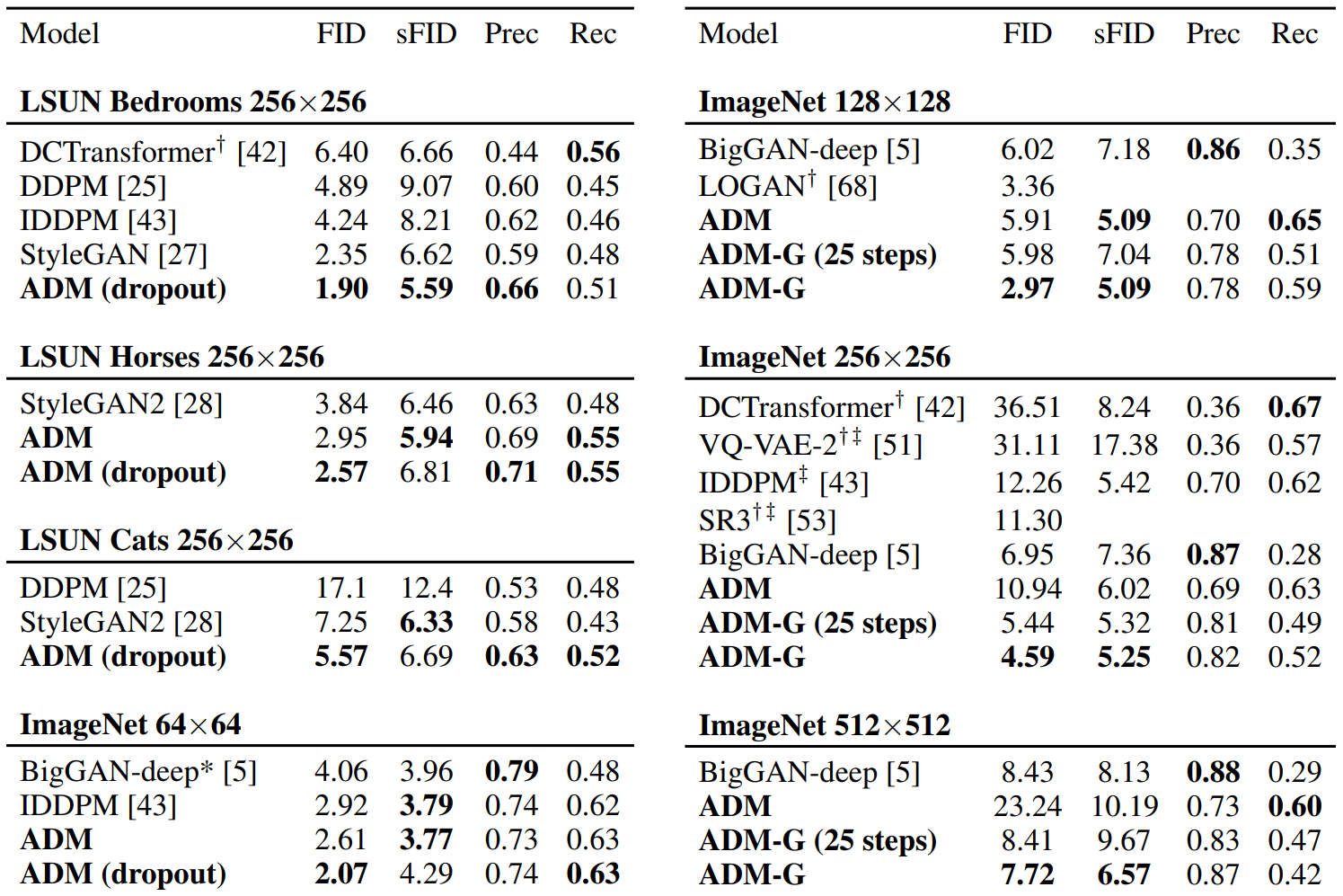
ADM은 ablated diffusion model의 약자이고, ADM-G는 추가로 classifier guidance를 사용한 모델이다. LSUN 모델은 1000 step으로 샘플링되었으며, ImageNet 모델은 250 step으로 샘플링되었다.

 ∗∗는 해상도에 맞는 BigGAN-deep 모델이 없어 저자들이 직접 학습시킨 모델이고, ††는 이전 논문에서 가져온 값들이다. ‡‡은 two-resolution stack을 사용한 결과이다.

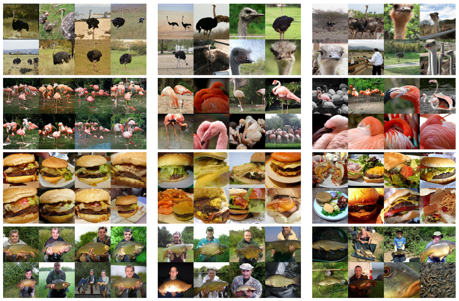
아래는 가장 성능이 좋은 BigGAN-deep 모델과 가장 성능이 좋은 저자들의 diffusion model의 임의의 샘플을 비교한 것이다.

5.2) Comparison to Upsampling

다음은 guidance와 two-stage upsampling stack의 비교이다. Upsampling model은 training set에서 이미지를 upsampling하고, 간단한 보간법을 사용하여 모델의 입력에 채널별로 연결되는 저해상도 이미지의 조건을 학습한다.

전체 샘플링은 저해상도 모델이 샘플을 생성한 다음 upsampling 모델이 이 샘플을 조건으로 사용하는 방식이다.

위의 표에서도 볼 수 있듯이, 이러한 방법을 사용하는 모델들은 ImageNet 256××256에서 FID가 개선되었지만 BigGAN-deep의 성능을 따라잡지 못하였다.

아래 표는 upsampling model과 guidance model을 비교한 표이다. Upsampling model은 Improved DDPM의 upsampling stack을 ADM에 적용한 것으로, ADM-U라 표기한다.

Classifier guidance와 upsampling을 결합하는 경우 해상도가 더 낮은 모델만 guide하였다.

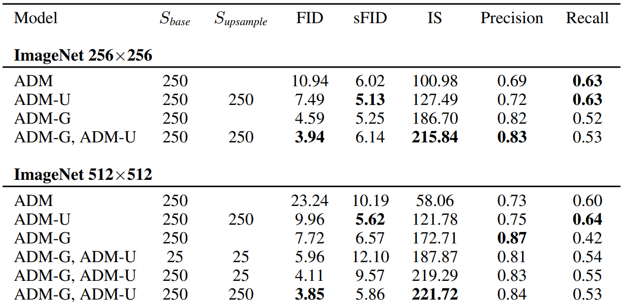
표에서 guidance와 upsampling이 서로 다른 방향으로 샘플의 품질을 향상시키는 것을 알 수 있다.

Upsampling은 recall을 높게 유지한 채로 precision을 개선하며, guidance는 훨씬 더 높은 precision을 위해 diversity를 절충할 수 있도록 한다.

7. Limitations

1. 여러 개의 denoising step을 사용하기 때문에 샘플링 시간에서 여전히 GAN보다 느리다.

• 이 방향에서 의미있는 논문 중 하나는 DDIM 샘플링 프로세스를 single step model로 distillation하는 방법을 연구한 Luhman과 Luhman의 논문이다.
• Single step model의 샘플은 아직 GAN과 경쟁력이 없지만 이전의 single-step likelihood-based model보다 훨씬 낫다.

2. 제안된 classifier guidance는 레이블이 있는 데이터셋에서만 사용할 수 있으며, 레이블이 없는 데이터셋의 fidelity를 위해 diversity를 교환하는 효과적인 전략은 아직 없다.