[Paper Review] Denoising Diffusion Probabilistic Model (DDPM)

이번에 리뷰할 논문은 DDPM이라 불리는 Denoising Diffusion Probabilistic Model이다.

해당 Paper는 아래의 링크에서 찾을 수 있다.

Denoising Diffusion Probabilistic Models

We present high quality image synthesis results using diffusion probabilistic models, a class of latent variable models inspired by considerations from nonequilibrium thermodynamics. Our best results are obtained by training on a weighted variational bound designed according to a novel connection between diffusion probabilistic models and denoising score matching with Langevin dynamics, and our models naturally admit a progressive lossy decompression scheme that can be interpreted as a generalization of autoregressive decoding. On the unconditional CIFAR10 dataset, we obtain an Inception score of 9.46 and a state-of-the-art FID score of 3.17. On 256x256 LSUN, we obtain sample quality similar to ProgressiveGAN. Our implementation is available at https://github.com/hojonathanho/diffusion

arXiv.orgJonathan Ho

보다 더 자세한 이해를 위해서는, 해당 post를 읽기 전에 Paper Preview글을 읽고 온다면 더욱 이해가 잘 될 것이다.

[Paper Preview] Denoising Diffusion Probabilistic Models

이번 DDPM을 Review하며 참고한 자료들은 다음과 같다. [개념 정리] Diffusion ModelGAN, VAE 와 같은 생성 모델(Generative Model) 중 하나로써, 2022년에 이슈가 되었던 text-to-image 모델인 Stable-Diffusion, DALL-E-2, Imagen의 기반이 되는 모델입니다. 많은 논문에서 Diffusion Model이 인용되지만 수식이 어려워서 간단하게 개념을 이해하고 넘어가기가 어렵습니다. 때문에 필요에 따라 깊이 별로 내용을 파악

Jaewon KimJaewon Kim

참고한 자료들은 다음과 같다.

What are Diffusion Models?

[Updated on 2021-09-19: Highly recommend this blog post on score-based generative modeling by Yang Song (author of several key papers in the references)]. [Updated on 2022-08-27: Added classifier-free guidance, GLIDE, unCLIP and Imagen. [Updated on 2022-08-31: Added latent diffusion model. [Updated on 2024-04-13: Added progressive distillation, consistency models, and the Model Architecture section. So far, I’ve written about three types of generative models, GAN, VAE, and Flow-based models. They have shown great success in generating high-quality samples, but each has some limitations of its own.

Lil'LogLilian Weng

[논문리뷰] Denoising Diffusion Probabilistic Models (DDPM)

DDPM 논문 리뷰 (NeurIPS 2020)

전생했더니 인공지능이었던 건에 대하여JiYeop Kim

ML simple works - A Gentle Introduction to Diffusion Model: Part 1 - DDPM

ML simple worksJo, Joonu (metamathgmail.com)

Diffusion Model 설명 - 기초부터 응용까지

Diffusion Model의 기초부터 응용까지 살펴봅니다. 기초 부분에서는 Diffusion Model의 동작 방법, Architecture, Loss Function을 살펴봅니다. 응용 부분에서는 다양한 Diffusion Model을 알아봅니다.

FFightingFfightingseok

[CVPR 2022] Diffusion Tutorials (Diffusion Basics, DDPM)

기존의 “CVPR 2022 Diffusion Tutorial” 에 관한 공식문서는 아래에서 확인할 수 있다. Denoising Diffusion-based Generative Modeling: Foundations and ApplicationsTutorial in Conjunction with CVPR 2023Denoising Diffusion-based Generative Modeling: Foundations and Applications 0. Diffusion Model [개념 정리] Diffusion ModelGAN, VAE 와 같은 생성 모델(Generative Model) 중 하나로써, 2022년에 이슈가 되었던 text-to-image

Jaewon KimJaewon Kim

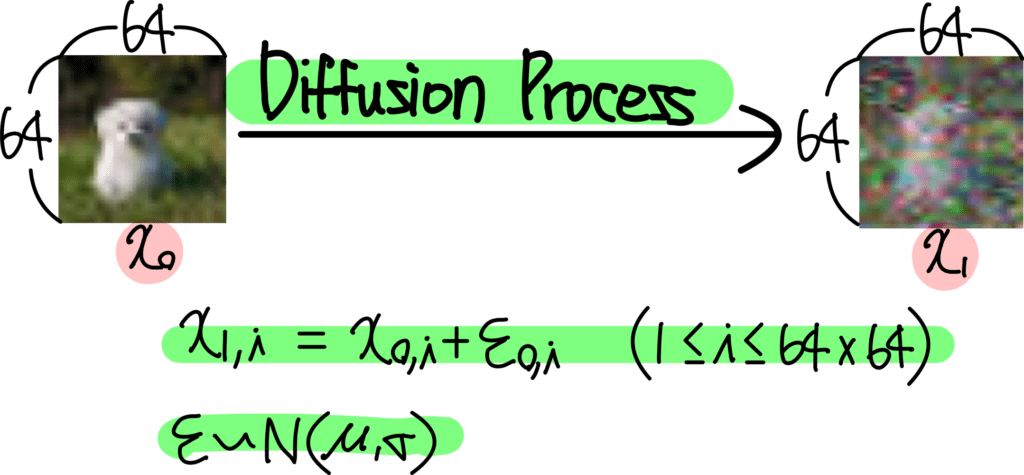
0. DDPM Preview

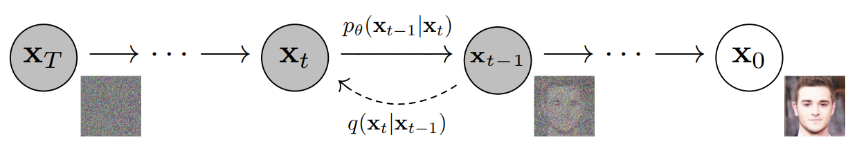
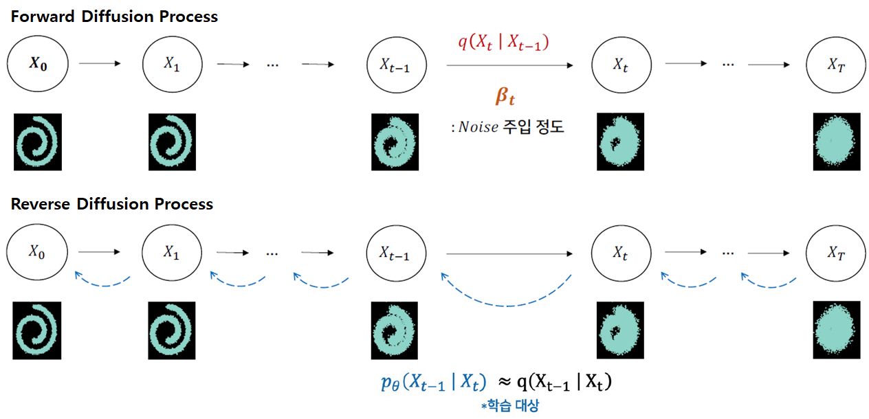
Forward Diffusion Process를 통해 매 time step마다 Input Image의 모든 pixel에 Gaussian Noise $\varepsilon_{\theta}$를 추가하고,

Reverse Denoising Process를 통해 매 time step마다 추가된 Gaussian Noise $\varepsilon_{\theta}$를 제거함으로써,

Input Image와 유사한 확률분포를 가지는 Result Image를 생성하는 모델이다.

Input Image에서 Gaussian Noise가 서서히 확산되기에 Diffusion(확산)이라는 이름이 붙었다고 한다.

• Forward Diffusion Process: Input Image에 fixed(고정된) Gaussian Noise가 더해진다.
• Reverse Denoising Process: Result Image에 learned(학습된) Gaussian Noise가 빼진다.

Diffusion Model의 목적은

Forward Diffusion Process를 거친 Result Image의 확률분포를 Reverse Denoising Process를 통해 Input(Real) Image의 확률분포와 유사하게 만드는 것이다.

이를 달성하기 위해 Reverse Denoising Process에서 학습을 통해 Noise 생성 확률 분포 Parameter인 Mean $\mu$, Standard Deviation $\sigma$를 조절한다.

"Diffusion"이라 함은 "확산" 현상을 의미한다.

아래의 그림을 보면 지정된 space안의 공기 분자들이 시간이 지남에 따라 Diffusion Process를 통해 전체 space안에 고르게 분포하는 것을 알 수 있다.

이때, 공기 분자 하나의 움직임을 관찰해보자.

매우 짧은 time step (sequence)동안 하나의 분자가 움직이는 Movement는 Gaussian Distribution을 따른다.

위의 그림은 매우 짧은 time step $t$ 단위로 분자 하나의 Movement $m_{t}$ 를 표시한 것이다. 이때, Movement $m_{t}$는 Gaussian Distribution을 따르므로 $m_{t} \sim N(\mu, \sigma)$으로 표현가능하다.

즉, 매시간 $t$마다 각 분자들은 Gaussian Distribution에 의한 Movement를 수행하는데 만약 이 Movement들을 예측해낼 수 있다면 Reverse Diffusion Process에 의해 Noisy 하지 않은 원상태를 구현할 수 있다.

이제, 위의 Diffusion Process를 Image에 적용해보자.

매 time step $t$마다 Molcule(분자)에 Gaussian Distribution을 따르는 Noise Movement $m_{t}$ 가 더해져 최종 Movement가 결정된다. 반면에 Image에서는 각 pixel에 Gaussian Noise $\varepsilon_{\theta}$ 가 더해져 그 다음 time step의 pixel이 된다.

위의 내용들을 종합하여 수식으로 나타내면 다음과 같다:

• $x_{0}$: 원본 image ($N \times N$ size)
• $x_{1}$: 다음 time step의 image
• $i$: image에 위치한 pixel의 position (index)

이미지의 각 pixel position에 대해 다음과 같이 식이 작성된다.

$x_{1, i}$ = $x_{0, i} + \varepsilon_{o, i}$ ($1 \leq i \leq N^{2}$)

$\varepsilon \sim N(\mu, \sigma)$

위의 예시는 $64 \times 64$의 image의 모든 pixel value에 Gaussian Noise $\varepsilon_{\theta}(x_{t}, t)$을 추가해주는 과정이다.

이러한 과정을 수많은 time step $t$ 마다 반복하여 완전한 Noise Image로 만들어준다. 이는 아래의 그림을 통해 설명가능하다.

위 과정은 Diffusion Forward Process라 한다. 매 time step $t$ 마다 이전 이미지 $x_{t-1}$의 모든 pixel에 fixed Gaussian Noise $\varepsilon$를 추가하여 time step $t$ 에서의 이미지 $x_{t}$를 형성한다.

위의 과정을 반복하여 최종 time step $T$에서는 $x_{T}$가 완전한 Noise Image가 되어있음을 알 수 있다.

이때, 매 time step $t$에서 첨가된 Gaussian Noise $\varepsilon_{\theta}(x_{t}, t)$을 계산할 수 있다면 Noise Image $x_{T}$에서 Real Image (Data) $x_{0}$로 Noise를 제거하면서(Subtraction) 되돌리는 것이 가능하다.

이는 Image Generation이 가능하다는 말을 뜻한다.

• Input: $x_{T}$ (random noise image)
• Output: $x_{0}$ (real / desired image)
• Process: Reverse Diffusion Process

정리해보면, Diffusion Model은 time step $t$에서의 image $x_{t}$를 입력으로 받아, 각 pixel별로 추가된 Gaussian Noise $\varepsilon_{\theta}(x_{t}, t)$를 예측하는 것이다.

해당 Noise $\varepsilon$를 subtract하면 이전 time step $t-1$에서의 image (less noisy image)로 변환가능하기에, $x_{T}$에서 위의 과정을 반복해 나가면 결국 real image (Data) $x_{0}$를 구현해낼 수 있다.

Diffusion Model이 갖춰야 하는 4가지 Condition들은 다음과 같다:

1. Input: Image or Noisy Image (3D Tensor 형태 or 2D Array 형태여야 한다)
2. Time step: 몇 번째 Process인지를 의미하는 $t$도 주어져야 한다.
3. Condition: 추가 Condition이 있다면 이 조건 또한 Diffusion Model에 주어져야 한다.
   1. Condition이란 특정 class 정보, 또는 생성한 이미지를 표현할 Text 정보 등등이 해당한다.
   2. Classifier Guidance를 통해 주어질 수도 있고, 바로 Diffusion Model에 주어질 수도 있다.
4. Output: Input과 동일한 Shape여야 한다.
   1. value는 각 pixel별로 첨가된 Noise값을 의미한다.
   2. Diffusion Model에 따라 Noise값 자체를 예측할지, Noise의 $\mu, \sigma$등을 예측할지는 조금씩 다르지만, Noise를 예측한다고 이해하면 큰 문제는 없다.

위 그림은 일반적인 Diffusion Model의 Architecture를 표현한 그림인데, Diffusion Model은 U-Net 구조를 띄고 있는 것을 알 수 있다.

• U-Net의 Structure 특성상 이는 Input과 동일한 Resoution을 가지는 Output을 내기에 용이하다.
• time step $t$ 를 별도로 입력받는다.
• 위의 구조는 대부분의 Diffusion Model에서 공통적으로 사용되고 있는 구조다.

앞서 말했듯, Diffusion Model은 time step $t$에서

• Input: Noisy Image $x_{t}$
• Output: Gaussian Noise $\varepsilon_{\theta}(x_{t}, t)$

위와 같음을 알 수 있다.

따라서, 각 pixel마다 첨가된 Gaussian Noise $\varepsilon_{\theta}$을 예측하는데, Loss Function은 아래와 같이 표현가능하다.

• $\varepsilon$: Ground Truth (Real Noise)
• $\varepsilon_{\theta}$: Diffusion Model이 예측한 Noise

위의 두 항이 같아지도록 Diffusion Model을 학습시킨다.

결국 DDPM 논문에서의 설명 Flow는 다음과 같다:

1) DDPM Loss 식을 간결화한다.

• VAE ELBO에서 Loss식 유도
• Regularization Term을 제거
• Denoising Matching Term 남김

2) $q(\mathbf{x}_{t-1}|\mathbf{x}_t,\mathbf{x}_0)$는 직접 유도하고, $p_{\theta}(\mathbf{x}_{t-1}|\mathbf{x}_{t})$는 Gaussian으로 모델링

Caution!

• $q(\mathbf{x}_{t-1}|\mathbf{x}_t,\mathbf{x}_0) = \mathcal{N}(\mathbf{x}_{t-1}; \tilde{\mu}_t(\mathbf{x}_t,\mathbf{x}_0), \tilde{\beta}_t I)$
  • Bayes' Rule을 통해 3개의 Gaussian을 다 전개하여 $\tilde{\mu}_t$, $\tilde{\beta}_t$에 대한 식을 직접 구함
  • Variance $\tilde{\beta}_t I$을 수식을 통해 직접 유도

• $p_{\theta}(\mathbf{x}_{t-1}|\mathbf{x}_{t}) = \mathcal{N}(\mathbf{x}_{t-1}; \mu_{\theta}(\mathbf{x}_t, t), \Sigma_{\theta}(\mathbf{x}_{t}, t))$
  • Variance $\Sigma_{\theta}$를 time-dependent constant로 fix 시킴
  • Mean $\mu_{\theta}$만 variable로 처리하여 Loss Function을 Simplify

즉, 실제로 Variance를 constant로 fix 시키는 부분은 $p_{\theta}(\mathbf{x}_{t-1}|\mathbf{x}_{t})$만 해당되는 것이다.

3) $p_{\theta}(\mathbf{x}_{t-1}|\mathbf{x}_{t})$의 Learnable Parameter $\mu_{\theta}(\mathbf{x}_t, t), \Sigma_{\theta}(\mathbf{x}_{t}, t))$ 중 $\mu_{\theta}(\mathbf{x}_t, t)$만 남긴다.

• $\Sigma_{\theta}(\mathbf{x}_{t}, t))$: Time-dependent Constant
• $\beta_t, \alpha_t$로 $\Sigma_{\theta}(\mathbf{x}_{t}, t))$ 표현가능

$$\sigma_{t}^{2} \cdot I = \tilde{\beta_{t}} \cdot I$$

4) Denoising Matching Term의 KL Divergence 두 분포가 Gaussian Distribution을 따른다.

• KLD의 두 distribution이 모두 gaussian 일 때 사용하는 공식
• constant를 제거하면 결국 두 $\mu$의 차에 의한 loss가 반환

$$\mathbb{E}_q\left[\frac{1}{2\sigma_t^2} ||\tilde{\mu_t}(x_t, x_0) - \mu_\theta(x_t, t)||^2\right]$$

5) $\mu_{\theta}(\mathbf{x}_t, t)$를 reparameterization trick을 이용하여 $\epsilon$에 대한 식으로 정리한다.

• 실제 각 time step $t$에서 정해져 있지 않은 항은 Gaussian Noise $\epsilon$뿐이다.
• 그렇기에 $\mu$에 대한 식을 $\epsilon$에 대한 식으로 재정리

$$\mathbb{E}_{x_0,\epsilon}\left[\frac{\beta_t^2}{2\sigma_t^2\alpha_t(1-\alpha_t)}\left|\epsilon - \epsilon_\theta\left(\sqrt{\alpha_t}x_0 + \sqrt{1-\alpha_t}\epsilon,t\right)\right|^2\right]$$

6) $\epsilon$에 대한 loss function을 정의하고, 상수 계수를 1로 처리한다.

• time step $t$가 증가함에 따라 계수가 점차 감소
• $t$가 큰 noisy image에 가까운 시점에서는 학습의 중요도가 앞의 작은 $t$에 비해 작음
• 따라서 계수를 상수로 만들어 상대적으로 $t$가 큰 시점에서의 학습의 중요도를 올림

$$L_\text{simple}(\theta) := \mathbb{E}_{t,x_0,\epsilon}\left[\left|\epsilon - \epsilon_\theta\left(\sqrt{\alpha_t}x_0 + \sqrt{1-\alpha_t}\epsilon,t\right)\right|^2\right]$$

1. Abstract

본 논문의 저자들은 Diffusion이라는 Probabilistic Generative Model을 nonequilibirum thermodynamics에서 영감을 받아, Diffusion Model을 이용하여 High-quality Image synthesis task를 수행한다.

Diffusion model은 class of latent variable ($\mathbf{x}_1, \mathbf{x}_2, ..., \mathbf{x}_T$)들을 사용한다.

이러한 DDPM Model의 best result는 weighted variational bound를 이용한 loss식을

1) DDPM과 denoising score matching term의 관계를 이용하여 novel한 변형을 가하고

2) Autoregressive decoding의 generalization으로 해석가능한 progressive lossy decompression을 수행한다.

2. Introduction

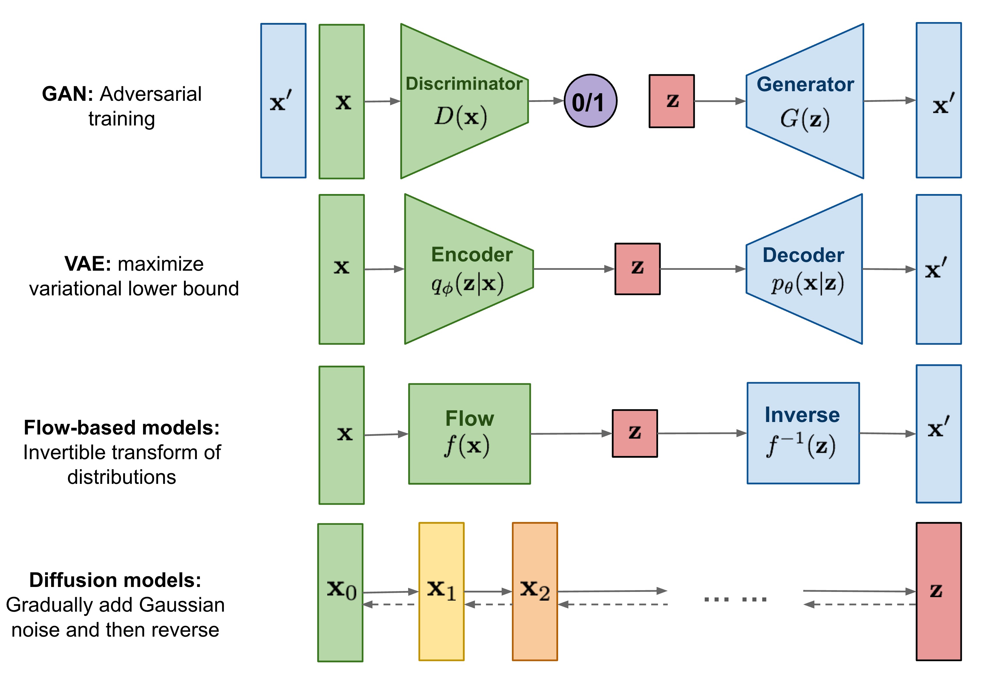
다수의 Probabilistic Generative Model들 (GAN, VAE, Flow-based, autoregressive 등)은 최근 폭넓은 variety를 가지는 high-quallity sample들을 생성하고 있다.

위의 Model들은 striking image, audio sample들을 생성할 뿐만 아니라, GAN에 비견될만한 image들을 생성하는 energy-based model이나 score matching 분야들도 놀라운 발전을 보이고 있다.

이 논문은 Diffusion probabilistic model에 대한 progress (DDPM) 를 다루고 있다.

DDPM 이전의 발전하기 전 논문은 아래의 링크에서 찾아볼 수 있다.

Deep Unsupervised Learning using Nonequilibrium Thermodynamics

A central problem in machine learning involves modeling complex data-sets using highly flexible families of probability distributions in which learning, sampling, inference, and evaluation are still analytically or computationally tractable. Here, we develop an approach that simultaneously achieves both flexibility and tractability. The essential idea, inspired by non-equilibrium statistical physics, is to systematically and slowly destroy structure in a data distribution through an iterative forward diffusion process. We then learn a reverse diffusion process that restores structure in data, yielding a highly flexible and tractable generative model of the data. This approach allows us to rapidly learn, sample from, and evaluate probabilities in deep generative models with thousands of layers or time steps, as well as to compute conditional and posterior probabilities under the learned model. We additionally release an open source reference implementation of the algorithm.

arXiv.orgJascha Sohl-Dickstein

Diffusion model은 parameterized된 markov chain을 variational inference를 이용하여 학습시켜 discrete time 이후 원하는 데이터에 맞는 sample을 생성하는 모델이다.

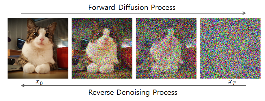
• Forward Diffusion Process: 점진적으로 data에 매 time step $t$마다 fixed gaussian noise를 주입하여 최종적으로는 data를 gaussian noise로 만든다. diffusion = noising = forward

• Reverse Denoising Process: Gaussian Noise에 매 time step $t$마다 learned gaussian noise를 제거하여 최종적으로는 input data와 유사한 확률분포를 가지는 data를 생성한다. sampling = denoising = reverse

Diffusion Model이 small amount of gaussian($\beta_t$) 으로 구성될 경우 sampling chain을 conditional gaussian으로 구성할 수 있으며, 간단한 neural network를 통해 parameterize할 수 있다.

Diffusion Model은 정의하기 쉽고 훈련하기 효율적이나, high-quality sample을 생성할 수 있는 능력에 대해서는 알려진 바가 없다.

본 논문의 저자들은 Diffusion Model이 high-quality image를 생성할 수 있으며, 다른 Generative model(e.g. GAN)보다 생성하는 result가 더 좋다고 주장한다.

또한 특정 paramterization이 훈련 중 다수의 noise level에서의 denoising score matching과 비슷하며, sampling(reverse) 중 Langevin dynamics 문제를 푸는 것과 동일하다고 말한다.

DDPM이 추가로 가지고 있는 특징은 다음과 같다:

• 1) Sample Quality가 좋음에도 불구하고 다른 likelihood-based model에 비해 competitive log-likelihood를 가지고 있지 않다.

• 2) DDPM의 대부분의 lossless codelength들이 인지할 수 없는 image detail을 설명하는데 사용되었다.

• 3) DDPM의 sampling procedure (reverse denoising)는 autoregressive decoding과 비슷한 progressive decoding이다.

3. Background

1) Prerequisite

Diffusion Model은 Input Data에 fixed noise를 추가하는 Forward Diffusion Process를 통해 Gaussian Noise를 만든 후,

Reverse Denoising Process를 통해 Gaussian Noise에서 Input Data의 distribution과 유사한 확률분포를 mapping하기 위해 subtract하는 Noise를 학습한다.

이때, Forward Diffusion Process는 fixed gaussian noise를 주입하기 때문에 $q(\mathbf{x}_{t}|\mathbf{x}_{t-1})$의 distribution은 알아서 결정된다.

다만, Reverse Denoising Process에서 사용되는 $q(\mathbf{x}_{t-1}|\mathbf{x}_{t})$는 Inference(generation)과정에서 사용이 불가능하다.

즉, $q(\mathbf{x}_{t}|\mathbf{x}_{t-1})$를 안다고 해서 direct하게 $q(\mathbf{x}_{t-1}|\mathbf{x}_{t})$으로의 변환이 불가능하다는 뜻이다.

왜 Reverse Process에서 $q(\mathbf{x}_{t-1}|\mathbf{x}_{t})$는 intractable한가?

Bayes' Rule에 의해 설명가능하다.

$$q(\mathbf{x}_{t-1}|\mathbf{x}_{t}) = \frac{q(\mathbf{x}_{t}|\mathbf{x}_{t-1})q(\mathbf{x}_{t-1})} {q(\mathbf{x}_{t})}$$

모든 time step $t$에 대한 $q(\mathbf{x}_t)$를 알아야 하므로 쉽지 않다.

따라서 Reverse Denoising process $q(\mathbf{x}_{t-1}|\mathbf{x}_{t})$가 neural network training을 통해 tractable한 $p_{\theta}(\mathbf{x}_{t-1}|\mathbf{x}_{t})$으로 대신 구현되어야 한다는 idea가 나온 것이다.

여기서 Forward/Reverse process모두 Gaussian Distribution을 따른다는 점이 반영된다.

여기서 $q(\mathbf{x}_{t-1}|\mathbf{x}_{t})$는 intractable하기에, $p_{\theta}(\mathbf{x}_{t-1}|\mathbf{x}_{t}) \approx q(\mathbf{x}_{t-1}|\mathbf{x}_{t})$를 만족하는 tractable한 $p_{\theta}(\mathbf{x}_{t-1}|\mathbf{x}_{t})$를 도입한다.

결국 Reverse Denoising Process를 통해 $p_{\theta}(\mathbf{x}_{t-1}|\mathbf{x}_{t}) \approx q(\mathbf{x}_{t-1}|\mathbf{x}_{t})$가 되도록 학습시킨다면,

subtract하는 gaussian noise를 예측할 수 있어 기존의 input data의 distribution과 유사한 distribution을 갖는 data를 생성할 수 있게 된다.

다만 이러한 transformation을 하나의 단일 step으로 표현하는 것은 매우 어려운 문제이다.

그렇기에 위의 step을 작은 step들로 잘게 나누어 학습한다.

따라서 Markov chain을 이용하여 discrete time step에서의 distribution을 곱함으로써, initial $\mathbf{x}_{0}$, 특정 $\mathbf{x}_{t}$ time step 간의 conditional distribution $q(\textbf{x}_{1:T} | \textbf{x}_{0}), p_{\theta}(\mathbf{x}_{0:T})$을 구할 수 있게 된다.

DDPM에서는 위의 step을 1000번으로 나누어 학습하며, 해당 과정인 $p_{\theta}(\mathbf{x}_{t-1}|\mathbf{x}_{t})$의 학습은 결국 estimating large number of small perturbations으로 볼 수 있다.

Markov Chain은 Markov 성질을 갖는 Dicrete한 확률과정이라 할 수 있다.

Discrete한 확률과정: Discrete Time $t=0, 1, 2, ...$ 속에서의 확률적 현상

여기서 Markov 성질이라 함은 "특정 상태($t+1$)의 확률은 오직 현재($t$)의 상태에만 의존한다." 으로 볼 수 있다.

$$q(\mathbf{x}_T|\mathbf{x}_{T-1}) = q(\mathbf{x}_T|\mathbf{x}_{T-1}, \mathbf{x}_{T-2}, ..., \mathbf{x}_1, \mathbf{x}_0)$$

2) Forward / Backward Process

Diffusion Model은 Reverse Desnoising Process를 통해 Gaussian Noise $\mathbf{x}_T$에서 매 time step $t$마다 학습되는 gaussian noise를 빼서,

최종적으로 initial time step $t_0$에 도달했을 때, input data의 확률분포와 유사한 분포를 가지는 data를 생성한다.

Diffusion Model은 아래와 같이 정의할 수 있다.

결국 Diffusion Model parameter $\theta$가 주어졌을 때 Reverse Denoising Process를 통해 우리가 원하는 정답인 input data $\mathbf{x}_0$가 나올 확률

$$p_{\theta}(\mathbf{x}_0) := \int p_{\theta}(\mathbf{x}_{0:T}) d\mathbf{x}_{1:T}$$

latent variable $\mathbf{x}_1, \mathbf{x}_2, ... ,\mathbf{x}_T$들은 모두 input data $\mathbf{x}_0$와 동일한 dimensionality를 갖는다.

Reverse Denoising Process는 joint distribution $p_{\theta}(\mathbf{x}_{0:T}) $으로 불린다.

이 Process는 $p(\mathbf{x}_T) = \mathcal{N}(\mathbf{x}_T; 0, I)$으로부터 시작하는 Markov Chain을 따른다.

• 1) $$p_{\theta}(\mathbf{x}_{0:T}) = p(\mathbf{x}_{T})\prod_{t=1}^{T} p_{\theta}(\mathbf{x}_{t-1}|\mathbf{x}_{t}) \qquad (1) $$

• 2) $$p_{\theta}(\mathbf{x}_{t-1}|\mathbf{x}_{t}) = \mathcal{N}(\mathbf{x}_{t-1}; \mu_{\theta}(\mathbf{x}_t, t), \Sigma_{\theta}(\mathbf{x}_{t}, t))$$

가 되는데, 이때 train해야 하는 parameter는 다음과 같다.

• $ \mu_{\theta}(\mathbf{x}_t, t)$: Mean
• $\Sigma_{\theta}(\mathbf{x}_{t}, t)$: Variance

두 개의 파라미터를 어떻게 Train시킬지가 굉장히 중요해진다.

Markov Chain에 의해 다음의 식이 성립한다:

$$\prod_{t=1}^{T} p_{\theta}(\mathbf{x}_{t-1}|\mathbf{x}_{t}) = p_\theta(x_0|x_1)p_\theta(x_1|x_2)p_\theta(x_2|x_3)...p_\theta(x_{T-1}|x_T)$$

$$= p_\theta(x_0|x_1,..., x_{T-1}, x_T)p_\theta(x_1 |x_2, ..., x_{T-1}, x_T)...p_\theta(x_{T-1}|x_T)$$

$$ = \frac{p_\theta(x_0,x_1,...,x_{T-1},x_T)}{p_\theta(x_1,...,x_{T-1},x_T)} \frac{p_\theta(x_1,...,x_{T-1},x_T)}{p_\theta(x_2,...,x_{T-1},x_T)}...\frac{p_\theta(x_{T-1},x_T)}{p_\theta(x_T)}$$

$$= \frac{p_\theta(x_0,x_1,...,x_{T-1},x_T)} {p_\theta(x_T)} = \frac{p_{\theta}(\mathbf{x}_{0:T})} {p_\theta(x_T)}$$

Forward Process: time step $t=0$에서 $t=T$로 갈수록 과거에서 미래로 간다고 해석한다.


Reverse Process: time step $t=T$에서 $t=0$로 갈수록 과거에서 미래로 간다고 해석한다.


따라서 Markov Chain의 성질을 적용할 때 주어진 Condition을 추가해도 되는 경우는 과거 의 경우에 한정하므로 Forward인지, Reverse인지 잘 구분해야 한다.

Forward Diffusion Process는 approximate posterior $q(\mathbf{x}_{1:T}|\mathbf{x}_0)$으로 불린다.

이 Process는 approximate posterior $q(\mathbf{x}_{1:T}|\mathbf{x}_0)$가 time step $t$에 따라 점진적으로 fixed gaussian noise $\beta_t$를 추가하는 markov chain이다.

• 1) $$\quad q(\mathbf{x}_{1:T}|\mathbf{x}_0) = \prod _{t=1}^T q(\mathbf{x}_t|\mathbf{x}_{t-1}) \qquad (2) $$

• 2) $$q(\textbf{x}_{t}|\textbf{x}_{t-1}) = N(\mathbf{x}_t ; \mu_{\mathbf{x}_t}, \Sigma_{\mathbf{x}_t} ) = N(\textbf{x}_{t}; \sqrt{1-\beta_{t}} \textbf{x}_{t-1}, \beta_{t}\textbf{I})$$

위와 같이 coefficient를 설정한 이유는 $Var(\mathbf{x}_0) = I$로 가정했을 때 $\mathbf{x}_t$의 Variance를 계속 $I$로 맞추기 위해서이다. (By reparameterization trick)

Markov 성질에 의해 $q(\mathbf{x}_T|\mathbf{x}_{T-1}) = q(\mathbf{x}_T|\mathbf{x}_{T-1}, \mathbf{x}_{T-2}, ..., \mathbf{x}_1, \mathbf{x}_0)$가 성립하여,

아래와 같이 식변형이 가능하다.

$$\quad q(\mathbf{x}_{1:T}|\mathbf{x}_0) = \prod _{t=1}^T q(\mathbf{x}_t|\mathbf{x}_{t-1}) = q(\mathbf{x}_1|\mathbf{x}_0)q(\mathbf{x}_2|\mathbf{x}_1)q(\mathbf{x}_3|\mathbf{x}_2)...q(\mathbf{x}_T|\mathbf{x}_{T-1}) $$

$$= q(\mathbf{x}_1|\mathbf{x}_0)q(\mathbf{x}_2|\mathbf{x}_1, \mathbf{x}_0)q(\mathbf{x}_3|\mathbf{x}_2, \mathbf{x}_1, \mathbf{x}_0)...q(\mathbf{x}_T|\mathbf{x}_{T-1}, .... , \mathbf{x}_1, \mathbf{x}_0)$$

$$= \frac{q(\mathbf{x}_1,\mathbf{x}_0)}{q(\mathbf{x}_0)} \frac{q(\mathbf{x}_2,\mathbf{x}_1,\mathbf{x}_0)}{q(\mathbf{x}_1,\mathbf{x}_0)}...\frac{q(\mathbf{x}_T,\mathbf{x}_{T-1},...,\mathbf{x}_1,\mathbf{x}_0)} {q(\mathbf{x}_{T-1},...,\mathbf{x}_0)}$$

$$= \frac{q(\mathbf{x}_0,\mathbf{x}_1,\mathbf{x}_2,\mathbf{x}_3,...,\mathbf{x}_T)}{q(\mathbf{x}_0)} = \quad q(\mathbf{x}_{1:T}|\mathbf{x}_0)$$

3) Diffusion Loss

Diffusion Model의 training은 negative log likelihood의 variational bound를 최적화하는 것으로 진행된다.

$$ \mathbb{E}_{q(\mathbf{x}_0)}[-\log p_\theta(\mathbf{x}_0)] \leq \mathbb{E}_{q(\mathbf{x}_{0:T})} \left[ -\log \left( \frac{p_\theta(\mathbf{x}_{0:T})}{q(\mathbf{x}_{1:T} | \mathbf{x}_0)} \right) \right] =\mathbb{E}_{q(\mathbf{x}_{0:T})} \left[ -\log p(\mathbf{x}_T) - \sum_{t=1}^T \log \frac{p_\theta(\mathbf{x}_{t-1} | \mathbf{x}_t)}{q(\mathbf{x}_t | \mathbf{x}_{t-1})} \right] := L \qquad(3) $$

실제 Diffusion Model은 다음과 같이 정의된다.

$$p_\theta(\mathbf{x}_0) = \int p_\theta(\mathbf{x}_{0:T})d\mathbf{x} _{1:T}$$

위의 식에서 $p_\theta(\mathbf{x}_0)$는 $\theta$에 대한 $\mathbf{x}_0$의 likelihood function이다.

Diffusion model parameter $\theta$를 조정해서 이 likelihood를 maximize 시키는 것을 MLE(Maximum Likelihood Estimation)이라 하며, 많은 모델들이 MLE 과정을 통해 학습하게 된다.

이렇듯 likelihood function $p_\theta(\mathbf{x}_0)$를 maximize시키는 parameter $\theta$를 최적화 알고리즘을 통해 찾는 것이 학습의 목표이다.

• likelihood function은 대체로 곱하기에 의해 정의되는 경우가 많으므로 likelihood $p_\theta(\mathbf{x}_0)$를 직접 다루기 보다 앞에 $\log$를 씌워서 log likelihood를 다룬다.
• Optimization의 경우 대체로 Minimization을 수행하므로 $-1$을 곱해서 $-\log$인 negative log likelihood로 만든다.

$$-\log p_\theta(\mathbf{x}_0) = -\log \left( \int p_\theta(\mathbf{x}_{0:T})d\mathbf{x}_{1:T} \right)$$

위의 식을 $\mathbf{x}_0$에 대한 conditional distribution $q(\mathbf{x}_{1:T}|\mathbf{x}_0)$에 대한 expectation으로 바꾸기 위해 우변을 다음처럼 변형한다.

어차피 적분변수가 $d\mathbf{x}_{1:T}$이므로 조건부 확률이어도 $|$ 앞 부분에 $\mathbf{x}_{1:T}$에 있다면 given condition은 상관없다.

$$ -\log p_\theta(\mathbf{x}_0) = -\log \left( \int p_\theta(\mathbf{x}_{0:T})d\mathbf{x}_{1:T} \right) $$

$$ = -\log \left( \int q(\mathbf{x}_{1:T} | \mathbf{x}_0) \frac{p_\theta(\mathbf{x}_{0:T})}{q(\mathbf{x}_{1:T} | \mathbf{x}_0)} d\mathbf{x}_{1:T} \right) $$

$$ = -\log \left( \mathbb{E}_{q(\mathbf{x}_{1:T}|\mathbf{x}_0)} \left[ \frac{p_\theta(\mathbf{x}_{0:T})}{q(\mathbf{x}_{1:T} | \mathbf{x}_0)} \right] \right) $$

위 식은 $\mathbf{x}_0$에 대한 likelihood는 $\frac{p_\theta(\mathbf{x}_{0:T})}{q(\mathbf{x}_{1:T} | \mathbf{x}_0)}$를 $\mathbf{x}_0$을 조건으로 하는 모든 존재 가능한 latent variable $\mathbf{x}_{1:T} | \mathbf{x}_0$에 대해 평균을 취한 것과 같다는 뜻이다.

$$ \leq \mathbb{E}_{q(\mathbf{x}_{1:T}|\mathbf{x}_0)} \left[ -\log \left( \frac{p_\theta(\mathbf{x}_{0:T})}{q(\mathbf{x}_{1:T} | \mathbf{x}_0)} \right) \right] $$

$-\log x$는 convex(볼록함수) function이므로 Jensen's Inequality가 성립한다. $$f(\mathbb{E}[x]) \leq \mathbb{E}[f(x)]$$

이제 위의 모든 항에 $\mathbb{E}_{q(\mathbf{x}_0)}$를 씌운다.

• $\mathbf{x} \leq \mathbf{y}$의 양변에 Expectation을 씌워도 부등식의 부등호 방향은 유지된다. $\mathbb{E}[\mathbf{x}] \leq \mathbb{E}[\mathbf{y}]$
• 어차피 양변에 probability space에 대한 integration을 수행하는 것이 Expectation이므로 부등호 방향은 유지될 수 밖에 없다.

Does taking expected value of two sides of inequality maintain the inequality?

As some operations are not necessarily valid for maintaining an inequality (such as raising both sides of $-2 < 2$ to an even power), I wondered if taking the expected value of both sides is act…

Mathematics Stack ExchangeFriedman

$$\mathbb{E}_{q(\mathbf{x}_0)}[-\log p_\theta(\mathbf{x}_0)] = \mathbb{E}_{q(\mathbf{x}_0)} \left[ -\log \left( \int p_\theta(\mathbf{x}_{0:T})d\mathbf{x}_{1:T} \right) \right] $$

$$ = \mathbb{E}_{q(\mathbf{x}_0)} \left[ -\log \left( \int q(\mathbf{x}_{1:T} | \mathbf{x}_0) \frac{p_\theta(\mathbf{x}_{0:T})}{q(\mathbf{x}_{1:T} | \mathbf{x}_0)} d\mathbf{x}_{1:T} \right) \right] $$

$$ = \mathbb{E}_{q(\mathbf{x}_0)} \left[ -\log \left( \mathbb{E}_{q(\mathbf{x}_{1:T}|\mathbf{x}_0)} \left[ \frac{p_\theta(\mathbf{x}_{0:T})}{q(\mathbf{x}_{1:T} | \mathbf{x}_0)} \right] \right) \right] $$

$$ \leq \mathbb{E}_{q(\mathbf{x}_0)} \left[ \mathbb{E}_{q(\mathbf{x}_{1:T}|\mathbf{x}_0)} \left[ -\log \left( \frac{p_\theta(\mathbf{x}_{0:T})}{q(\mathbf{x}_{1:T} | \mathbf{x}_0)} \right) \right] \right] $$

$$ = \mathbb{E}_{q(\mathbf{x}_{0:T})} \left[ -\log \left( \frac{p_\theta(\mathbf{x}_{0:T})}{q(\mathbf{x}_{1:T} | \mathbf{x}_0)} \right) \right] $$

맨 마지막에 등호가 성립하는 이유는 다음과 같다.

Joint Distribution에 대한 Expectation을 likelihood와 prior의 대한 Expectation의 합성 형태로 작성할 수 있다.

즉, 정리하면 다음의 식이 성립한다.

$$ \mathbb{E}_{q(\mathbf{x}_0)}[-\log p_\theta(\mathbf{x}_0)] \leq \mathbb{E}_{q(\mathbf{x}_{0:T})} \left[ -\log \left( \frac{p_\theta(\mathbf{x}_{0:T})}{q(\mathbf{x}_{1:T} | \mathbf{x}_0)} \right) \right] \qquad (3*) $$

위의 식 $(3*)$은 input data $\mathbf{x}_0$의 $\theta$에 대한 negative log likelihood는 우변의 Variational Bound보다 클 수 없다는 것을 의미한다.

Variational Bound라는 단어를 사용하는 이유는 해당 상한은 latent variable의 distribution으로 제안된 함수 $q(\mathbf{x}_{1:T} | \mathbf{x}_0)$에 따라 달라지기 때문이다.

즉, 해당 Variational Bound가 상한이므로 우변을 $\theta$에 대해 Minimize하면 좌변은 항상 우변보다 더 작아지게 된다.

다시 말해, 이 Variational Bound를 Loss Function으로 사용할 수 있게 되는 것이다.

이제 유도된 ELBO를 $\theta$에 대해 optimize하는 것이 목적이므로, $\theta$에 대한 항과 없는 항으로 분리한다.

$$-\log \left( \frac{p_\theta(\mathbf{x}_{0:T})}{q(\mathbf{x}_{1:T} | \mathbf{x}_0)} \right) = -\log \left( \frac{p(\mathbf{x}_T) \prod_{t=1}^T p_\theta(\mathbf{x}_{t-1} | \mathbf{x}_t)}{\prod_{t=1}^T q(\mathbf{x}_t | \mathbf{x}_{t-1})} \right) $$

$$ = -\log \left( p(\mathbf{x}_T) \cdot \frac{\prod_{t=1}^T p_\theta(\mathbf{x}_{t-1} | \mathbf{x}_t)}{\prod_{t=1}^T q(\mathbf{x}_t | \mathbf{x}_{t-1})} \right) $$

$$ = -\log p(\mathbf{x}_T) - \log \prod_{t=1}^T \frac{p_\theta(\mathbf{x}_{t-1} | \mathbf{x}_t)}{q(\mathbf{x}_t | \mathbf{x}_{t-1})} $$

$$ = -\log p(\mathbf{x}_T) - \sum_{t=1}^T \log \frac{p_\theta(\mathbf{x}_{t-1} | \mathbf{x}_t)}{q(\mathbf{x}_t | \mathbf{x}_{t-1})}$$

따라서 전개된 부분을 다시 원식에 적용하면 맨 처음에 제시한 식 $(3)$이 완성된다.

최종적으로 가장 오른쪽에 있는 항을 Loss Function $L$로 정의하게 된다.

$$ \mathbb{E}_{q(\mathbf{x}_0)}[-\log p_\theta(\mathbf{x}_0)] \leq \mathbb{E}_{q(\mathbf{x}_{0:T})} \left[ -\log \left( \frac{p_\theta(\mathbf{x}_{0:T})}{q(\mathbf{x}_{1:T} | \mathbf{x}_0)} \right) \right] =\mathbb{E}_{q(\mathbf{x}_{0:T})} \left[ -\log p(\mathbf{x}_T) - \sum_{t=1}^T \log \frac{p_\theta(\mathbf{x}_{t-1} | \mathbf{x}_t)}{q(\mathbf{x}_t | \mathbf{x}_{t-1})} \right] := L \qquad(3) $$

EM Algorithm을 통해 ELBO에 대한 부등식으로 정리하고, 이를 Maximize 시킨다.

data $\mathbf{x}_0$에 대한 likelihood는 다음처럼 분해될 수 있다.

$$\log p_\theta(\mathbf{x}_0) = \mathbb{E}_{q(\mathbf{x}_{1:T})} \left[ \log \frac{p_\theta(\mathbf{x}_{0:T})}{q(\mathbf{x}_{1:T})} \right] + \left( -\mathbb{E}_{q(\mathbf{x}_{1:T})} \left[ \log \frac{p_\theta(\mathbf{x}_{1:T} | \mathbf{x}_0)}{q(\mathbf{x}_{1:T})} \right] \right)$$

위와 같이 분해가 가능한 이유는 EM Algorithm에 의해서이다. 더 자세한 내용을 알고 싶다면 아래의 링크를 참고하자.

$$ln p(\mathbf{x}|\theta) = \mathcal{L}(q, \theta) + D_{KL}(q \parallel p)$$

ML simple works - A Step by Step Introduction to EM Algorithm

ML simple worksJo, Joonu (metamathgmail.com)

이렇게 분해된 우변의 첫 번째 항을 Variational Low Bound 혹은 ELBO(Evidence Lower Bound)라 부르고, 두 번째 항은 KL Divergence라 한다.

• KL Divergence는 두 확률분포의 차이를 측정하는 값으로 해석이 가능하다.
• 위 식의 두 번째 항인 KLD는 다음과 같이 볼 수 있다. $D_{KL}(q(\mathbf{x}_{1:T} \parallel p_\theta(\mathbf{x}_{1:T} | \mathbf{x}_0))) \geq 0$

따라서 위 등식은 아래와 같은 부등식으로의 변형이 가능하다.

$$\log p_\theta(\mathbf{x}_0) \geq \mathbb{E}_{q(\mathbf{x}_{1:T})} \left[ \log \frac{p_\theta(\mathbf{x}_{0:T})}{q(\mathbf{x}_{1:T})} \right]$$

우변의 $q(\mathbf{x}_{1:T})$는 latent variable $\mathbf{x}_{1:T}$의 분포에 대해 알지 못하기에 임의로 제안된 분포이다.


latent variable에 대한 분포를 어떠한 분포로 제안을 해도 위 식이 성립한다.

$$ \log p_\theta(\mathbf{x}_0) = \mathbb{E}_{q(\mathbf{x}_{1:T})} \left[ \log \frac{p_\theta(\mathbf{x}_{0:T})}{q(\mathbf{x}_{1:T})} \right] + D_{KL} $$

따라서 위의 분해식에서 distribution을 $q(\mathbf{x}_{1:T})$에서 $q(\mathbf{x}_{1:T} | \mathbf{x}_0)$으로 제안한다.

$$ \log p_\theta(\mathbf{x}_0) = \mathbb{E}{q(\mathbf{x}_{1:T}|\mathbf{x}_0)} \left[ \log \frac{p_\theta(\mathbf{x}_{0:T})}{q(\mathbf{x}_{1:T} | \mathbf{x}_0)} \right] + D_{KL} $$

$$ \mathbb{E}_{q(\mathbf{x}_0)}[\log p_\theta(\mathbf{x}_0)] \geq \mathbb{E}_{q(\mathbf{x}_{0:T})} \left[ \log \frac{p_\theta(\mathbf{x}_{0:T})}{q(\mathbf{x}_{1:T} | \mathbf{x}_0)} \right] $$

위 식은 식 $(3*)$과 부등호 방향을 제외하고 전부 동일하다.

우변을 $\theta$에 대해 Maximize 하게 되면 lower bound가 커져 좌변은 maximized된 우변보다 항상 조금 더 커지게 되고, 그 차이가 0이상인 $D_{KL}$로 나타나게 되는 것이다.

식 $(3*)$에서도 동일한 논리가 적용되는데, 다른 점은 lower bound가 upper bound로 바뀌어 있기 때문에 우변을 Minimize하면 좌변은 항상 우변보다 더 작아지게 된다.

따라서 식 $(3*)$의 upper bound를 Loss Function $L$로 사용이 가능한 것이다.

• Forward Process: $\beta_t$는 reparameterization으로 학습하거나 constant로 처리할 수 있다.
• Reverse Process: $p_{\theta}(\mathbf{x}_{t} | \mathbf{x}_{t-1})$의 gaussian condition의 선택에 따라 부분적으로 보장된다.

$\beta_t$가 충분히 작으면 Forward $q(\mathbf{x}_{t} | \mathbf{x}_{t-1})$와 Reverse $p_{\theta}(\mathbf{x}_{t} | \mathbf{x}_{t-1})$는 모두 Gaussian Distribution을 따른다.

4) Reparameterization Trick

forward process의 주목할만한 점은 closed form의 형태로 임의의 time step $t$에서 $\mathbf{x}_t$의 sampling을 바로 할 수 있다는 점이다.

$$q(\mathbf{x}_t|\mathbf{x}_0) = \mathcal{N}(\mathbf{x}_t; \sqrt{\bar{\alpha}_t}\mathbf{x}_0, (1 - \bar{\alpha}_t)\mathbf{I})$$


$$\alpha_t = 1 - \beta_t \: \text{and} \: \bar{\alpha}_{t} = \prod_{s=1}^{t} \alpha_s$$

그렇다면 위의 식과 같이 임의의 time step $t$에서 $\mathbf{x}_t$의 sampling을 바로 할 수 있는 것이 왜 필요할까?

앞서 정의했던 Loss Function $L$을 다시 살펴보자.

$$ \mathbb{E}_{q(\mathbf{x}_{0:T})} \left[ -\log p(\mathbf{x}_T) - \sum_{t=1}^T \log \frac{p_\theta(\mathbf{x}_{t-1} | \mathbf{x}_t)}{q(\mathbf{x}_t | \mathbf{x}_{t-1})} \right] := L \qquad(3) $$

이를 계산하기 위해서는 임의의 sample $\mathbf{x}_0$를 선택하고 이로부터 noise를 확산시켜 $\mathbf{x}_1, \mathbf{x}_2, ... , \mathbf{x}_T$를 얻는다.

이 과정에서 $q(\mathbf{x}_t | \mathbf{x}_{t-1})$를 단계적으로 계산해야 했다. 즉, $q(\mathbf{x}_t | \mathbf{x}_{t-1})$를 계산하기 위해 $q(\mathbf{x}_{t-1} | \mathbf{x}_{t-2}), ... , q(\mathbf{x}_{1} | \mathbf{x}_{0})$를 반드시 거쳐야만 했다.

따라서 임의의 time step $t$에 대해서 $q(\mathbf{x}_t | \mathbf{x}_{0})$를 바로 정의할 수 있다면 임의의 time step $t$ 에서의 noise가 확산된 sample을 바로 얻을 수 있어 학습의 효율을 높일 수 있다.

$q(\mathbf{x}_t | \mathbf{x}_{0})$는 $q(\mathbf{x}_t | \mathbf{x}_{t-1})$의 정의와 Reparameterization Trick을 사용하면 얻을 수 있다.

$q(\mathbf{x}_t | \mathbf{x}_{t-1})$는 다음과 같이 정의가능하다.

$q(\mathbf{x}_t | \mathbf{x}_{t-1}) := N(\mathbf{x}_t ; \mu_{\mathbf{x}_{t-1}}, \Sigma_{\mathbf{x}_{t-1}}) := N(\mathbf{x}_t ; \sqrt{1-\beta_t} \mathbf{x}_{t-1}, \beta_t I)$

이때, $\alpha_t = 1 - \beta_t$ and $\bar{\alpha}_{t} = \prod_{s=1}^{t} \alpha_s$라 한다면,

$X$가 Gaussian Distribution을 따를 때, 아래의 Reparameterization Trick을 사용할 수 있다.

따라서, $\mathbf{x}_{t}$는 다음과 같이 정의할 수 있다.

$\mathbf{x}_{t} = \sqrt{\alpha_{t}}\mathbf{x}_{t-1} + \sqrt{1-\alpha_{t}}\epsilon_{t-1} \quad \text{;where } \epsilon_{t-1}, \epsilon_{t-2}, \cdots \sim \mathcal{N}(0, \mathbf{I})$

이제 $\mathbf{x}_{t-1}$의 자리에 순서대로 역대입을 하여 계산을 하면,

$$\mathbf{x}_{t} = \sqrt{\alpha_t}\mathbf{x}_{t-1} + \sqrt{1-\alpha_{t}}\epsilon_{t-1} \quad \text{;where } \epsilon_{t-1}, \epsilon_{t-2}, \cdots \sim \mathcal{N}(0, \mathbf{I})$$

$$ = \sqrt{\alpha_t} \left(\sqrt{\alpha_{t-1}} \mathbf{x}_{t-2} + \sqrt{1-\alpha_{t-1}}\epsilon_{t-2} \right) + \sqrt{1-\alpha_{t}}\epsilon_{t-1}$$

$$ = \sqrt{\alpha_t \alpha_{t-1}}\mathbf{x}_{t-2} + \sqrt{\alpha_t}\sqrt{1-\alpha_{t-1}}\epsilon_{t-2} + \sqrt{1-\alpha_{t}}\epsilon_{t-1}$$

$$\sqrt{\alpha_t}\sqrt{1-\alpha_{t-1}}\epsilon_{t-2} \sim \mathcal{N}\left(0, \alpha_t(1-\alpha_{t-1})\mathbf{I}\right)$$
$$\sqrt{1-\alpha_{t}}\epsilon_{t-1} \sim \mathcal{N}\left(0, (1-\alpha_{t})\mathbf{I}\right)$$

이때, 마지막 2개 항은 각각 평균 $\mu$이 0인 Gaussian Distribution을 따르고 있으며 2개의 Gaussian은 아래의 공식에 따라 Merge할 수 있다.

$$X \sim \mathcal{N}(\mu_X, \sigma_X^2)$$
$$Y \sim \mathcal{N}(\mu_Y, \sigma_Y^2)$$
$$X + Y \sim \mathcal{N}(\mu_X + \mu_Y, \sigma_X^2 + \sigma_Y^2)$$

이에 대한 증명은 아래에서 찾아볼 수 있다.

Sum of normally distributed random variables - Wikipedia

Wikimedia Foundation, Inc.Contributors to Wikimedia projects

$$\sqrt{\alpha_t}\sqrt{1-\alpha_{t-1}}\epsilon_{t-2} + \sqrt{1-\alpha_{t}}\epsilon_{t-1} \sim \mathcal{N}\left(0, \left(\alpha_t(1-\alpha_{t-1}) + (1-\alpha_{t})\right)\mathbf{I}\right)$$

$$= \sqrt{\alpha_t\alpha_{t-1}}\mathbf{x}_{t-2} + \sqrt{1-\alpha_t\alpha_{t-1}}\epsilon_{t-2}^{*} \quad \text{;where } \epsilon_{t-2}^{*} \text{ merges two Gaussians (*).}$$

$$= \cdots$$

$$ = \sqrt{\bar{\alpha}_t}\mathbf{x}_0 + \sqrt{1-\bar{\alpha}_t}\epsilon \quad \text{where} \quad \alpha_t = 1 - \beta_t \: \text{and} \: \bar{\alpha}_{t} = \prod_{s=1}^{t} \alpha_s$$

위와 같이 정리할 수 있으며, 결과적으로 아래와 같은 식을 도출할 수 있다.

$$q(\mathbf{x}_t|\mathbf{x}_0) = \mathcal{N}(\mathbf{x}_t; \sqrt{\bar{\alpha}_t}\mathbf{x}_0, (1 - \bar{\alpha}_t)\mathbf{I}), \quad \alpha_t = 1 - \beta_t \: \text{and} \: \bar{\alpha}_{t} = \prod_{s=1}^{t} \alpha_s$$

이로써 time step을 처음부터 시작하지 않고도 건너뛰며 빠르게 noise를 추가할 수 있게 되었다.

sampling이 훨씬 빠르게 가능해졌으므로, 이 sample들을 이용하여 효율적으로 Loss Function $L$에 나타나는, $p_\theta(\mathbf{x}_{t-1} | \mathbf{x}_t)$와 $q(\mathbf{x}_t | \mathbf{x}_{t-1})$를 계산할 수 있게 되었다.

• $p_\theta(\mathbf{x}_{t-1} | \mathbf{x}_t) := \mathcal{N}(\mathbf{x}_{t-1}; \mu_\theta(\mathbf{x}_t, t), \Sigma_\theta(\mathbf{x}_t, t))$
• $q(\mathbf{x}_t | \mathbf{x}_{t-1}) := \mathcal{N}(\mathbf{x}_t; \sqrt{1 - \beta_t}\mathbf{x}_{t-1}, \beta_t\mathbf{I})$

5) DDPM Loss

DDPM에서는 아래 $(3)$과 같이 유도된 Loss Function $L$을 바로 사용하지 않고, 한 번 더 형태를 변형하여 더 간결하게 $(5)$로 만든다.

$$ \mathbb{E}_{q(\mathbf{x}_0)}[-\log p_\theta(\mathbf{x}_0)] \leq \mathbb{E}_{q(\mathbf{x}_{0:T})} \left[ -\log \left( \frac{p_\theta(\mathbf{x}_{0:T})}{q(\mathbf{x}_{1:T} | \mathbf{x}_0)} \right) \right] =\mathbb{E}_{q(\mathbf{x}_{0:T})} \left[ -\log p(\mathbf{x}_T) - \sum_{t=1}^T \log \frac{p_\theta(\mathbf{x}_{t-1} | \mathbf{x}_t)}{q(\mathbf{x}_t | \mathbf{x}_{t-1})} \right] := L \qquad(3) $$

$$L = \mathbb{E}_{q(\mathbf{x}_{0:T})}\left[D_{KL}(q(\mathbf{x}_T | \mathbf{x}_0)||p(\mathbf{x}_T)) + \sum_{t=2}^T D_{KL}(q(\mathbf{x}_{t-1} | \mathbf{x}_t, \mathbf{x}_0)||p_\theta(\mathbf{x}_{t-1} |\mathbf{x}_t))-\log p_\theta(\mathbf{x}_0 | \mathbf{x}_1)\right] \qquad (5)$$

우선, sampling을 더 빠르게 하기 위해, Loss Function의 분모에 있는 $q(\mathbf{x}_t | \mathbf{x}_{t-1})$항을 위에서 언급한 $q(\mathbf{x}_t|\mathbf{x}_0)$에 대한 식으로 변형해야 한다.

따라서 Forward Diffusion Process을 구성하는 $q(\mathbf{x}_t | \mathbf{x}_{t-1})$ 항을 Bayes' Rule과 Makov 성질에 의해 다음과 같이 작성할 수 있다.

$$q(\mathbf{x}_t | \mathbf{x}_{t-1}) = q(\mathbf{x}_t | \mathbf{x}_{t-1}, \mathbf{x}_{0}) = \frac{q(\mathbf{x}_{t-1} | \mathbf{x}_t, \mathbf{x}_0)q(\mathbf{x}_t, \mathbf{x}_0)}{q(\mathbf{x}_{t-1}, \mathbf{x}_0)}= \frac{q(\mathbf{x}_{t-1} | \mathbf{x}_t, \mathbf{x}_0)q(\mathbf{x}_t |\mathbf{x}_0)}{q(\mathbf{x}_{t-1} | \mathbf{x}_0)}$$

이 결과를 위의 Loss Function의 $\log \frac{p_\theta(\mathbf{x}_{t-1} | \mathbf{x}_t)}{q(\mathbf{x}_t | \mathbf{x}_{t-1})}$ 항에 대입한다.

$$\log \frac{p_\theta(\mathbf{x}_{t-1} | \mathbf{x}_t)}{q(\mathbf{x}_t | \mathbf{x}_{t-1})} = \log \frac{p_\theta(\mathbf{x}_{t-1} | \mathbf{x}_t)}{\frac{q(\mathbf{x}_{t-1} | \mathbf{x}_t, \mathbf{x}_0)q(\mathbf{x}_t | \mathbf{x}_0)}{q(\mathbf{x}_{t-1} | \mathbf{x}_0)}}$$

$$= \log \frac{p_\theta(\mathbf{x}_{t-1} | \mathbf{x}_t)}{q(\mathbf{x}_{t-1} | \mathbf{x}_t, \mathbf{x}_0)} \cdot \frac{q(\mathbf{x}_{t-1} | \mathbf{x}_0)}{q(\mathbf{x}_t | \mathbf{x}_0)}$$

위 식의 결과를 $(3)$에 대입하고 정리하자.

$$L = \mathbb{E}_{q(\mathbf{x}_{0:T})} \left[-\log \left(\frac{p_\theta(\mathbf{x}_{0:T})}{q(\mathbf{x}_{1:T} | \mathbf{x}_0)}\right)\right]$$

$$= \mathbb{E}_{q(\mathbf{x}_{0:T})} \left[-\log p(\mathbf{x}_T) - \sum_{t=1}^T \log \frac{p_\theta(\mathbf{x}_{t-1} | \mathbf{x}_t)}{q(\mathbf{x}_t | \mathbf{x}_{t-1})}\right]$$

여기서 $t=1$일 때와 $t \geq 2$ 일 때로 나눈다.

$$= \mathbb{E}_{q(\mathbf{x}_{0:T})} \left[-\log p(\mathbf{x}_T) - \sum_{t=2}^T \log \frac{p_\theta(\mathbf{x}_{t-1} | \mathbf{x}_t)}{q(\mathbf{x}_t | \mathbf{x}_{t-1})} - \log \frac{p_\theta(\mathbf{x}_0 | \mathbf{x}_1)}{q(\mathbf{x}_1 | \mathbf{x}_0)}\right]$$

위의 결과를 이제 $\log$ 식의 분모에 대입해서 정리한다.

$$= \mathbb{E}_{q(\mathbf{x}_{0:T})} \left[-\log p(\mathbf{x}_T) - \sum_{t=2}^T \log \frac{p_\theta(\mathbf{x}_{t-1} | \mathbf{x}_t)}{q(\mathbf{x}_{t-1} | \mathbf{x}_t, \mathbf{x}_0)} \cdot \frac{q(\mathbf{x}_{t-1} | \mathbf{x}_0)}{q(\mathbf{x}_t | \mathbf{x}_0)} - \log \frac{p_\theta(\mathbf{x}_0 | \mathbf{x}_1)}{q(\mathbf{x}_1 | \mathbf{x}_0)}\right]$$

결국 Loss Function $L$은 다음과 같이 나온다.

$$L = \mathbb{E}_{q(\mathbf{x}_{0:T})} \left[-\log p(\mathbf{x}_T) - \sum_{t=2}^T \log \frac{p_\theta(\mathbf{x}_{t-1} | \mathbf{x}_t)}{q(\mathbf{x}_{t-1} | \mathbf{x}_t, \mathbf{x}_0)} \cdot \frac{q(\mathbf{x}_{t-1} | \mathbf{x}_0)}{q(\mathbf{x}_t | \mathbf{x}_0)} - \log \frac{p_\theta(\mathbf{x}_0 | \mathbf{x}_1)}{q(\mathbf{x}_1 | \mathbf{x}_0)}\right]$$

$$= \mathbb{E}_{q(\mathbf{x}_{0:T})} \left[-\log p(\mathbf{x}_T) - \sum_{t=2}^T \log \frac{p_\theta(\mathbf{x}_{t-1} | \mathbf{x}_t)}{q(\mathbf{x}_{t-1} | \mathbf{x}_t, \mathbf{x}_0)} - \sum_{t=2}^T \log \frac{q(\mathbf{x}_{t-1} | \mathbf{x}_0)}{q(\mathbf{x}_t | \mathbf{x}_0)} - \log \frac{p_\theta(\mathbf{x}_0 | \mathbf{x}_1)}{q(\mathbf{x}_1 | \mathbf{x}_0)}\right]$$

여기서 아래의 항은 Telescoping을 통해 다음과 같이 정리된다.


$$-\sum_{t=2}^T \log \frac{q(\mathbf{x}_{t-1} | \mathbf{x}_0)}{q(\mathbf{x}_t | \mathbf{x}_0)} = - \log \frac{q(\mathbf{x}_{1} | \mathbf{x}_0)}{q(\mathbf{x}_T | \mathbf{x}_0)}$$


항 1개 차이이므로 앞의 항에 큰 값, 뒤의 항에 작은 값 (큰큰작작)을 넣어주어 간단하게 정리한다.

$$= \mathbb{E}_{q(\mathbf{x}_{0:T})} \left[-\log p(\mathbf{x}_T) - \sum_{t=2}^T \log \frac{p_\theta(\mathbf{x}_{t-1} | \mathbf{x}_t)}{q(\mathbf{x}_{t-1} | \mathbf{x}_t, \mathbf{x}_0)} - \log \frac{q(\mathbf{x}_{1} | \mathbf{x}_0)}{q(\mathbf{x}_T | \mathbf{x}_0)} - \log \frac{p_\theta(\mathbf{x}_0 | \mathbf{x}_1)}{q(\mathbf{x}_1 | \mathbf{x}_0)}\right]$$

$$= \mathbb{E}_{q(\mathbf{x}_{0:T})} \left[-\log \frac{p(\mathbf{x}_T)}{q(\mathbf{x}_T | \mathbf{x}_0)} - \sum_{t=2}^T \log \frac{p_\theta(\mathbf{x}_{t-1} | \mathbf{x}_t)}{q(\mathbf{x}_{t-1} | \mathbf{x}_t, \mathbf{x}_0)} - \log p_\theta(\mathbf{x}_0 | \mathbf{x}_1)\right]$$

결국 최종 Loss $L$은 다음과 같이 정리할 수 있다.

$$L = \mathbb{E}_{q(\mathbf{x}_{0:T})} \left[-\log \frac{p(\mathbf{x}_T)}{q(\mathbf{x}_T | \mathbf{x}_0)} - \sum_{t=2}^T \log \frac{p_\theta(\mathbf{x}_{t-1} | \mathbf{x}_t)}{q(\mathbf{x}_{t-1} | \mathbf{x}_t, \mathbf{x}_0)} - \log p_\theta(\mathbf{x}_0 | \mathbf{x}_1)\right]$$

Expectation 연산을 쪼갠 후에, 각 항을 KL Divergence $D_{KL}$ 형태로 변형한다.

$$= \mathbb{E}_{q(\mathbf{x}_{0:T})} \left[-\log \frac{p(\mathbf{x}_T)}{q(\mathbf{x}_T | \mathbf{x}_0)}\right] + \mathbb{E}_{q(\mathbf{x}_{0:T})} \left[-\sum_{t=2}^T \log \frac{p_\theta(\mathbf{x}_{t-1} | \mathbf{x}_t)}{q(\mathbf{x}_{t-1} | \mathbf{x}_t, \mathbf{x}_0)}\right] + \mathbb{E}_{q(\mathbf{x}_{0:T})} [-\log p_\theta(\mathbf{x}_0 | \mathbf{x}_1)]$$

Joint Distribution에 대한 Expectation을 likelihood와 prior의 대한 Expectation의 합성 형태로 작성할 수 있다.

$$= \mathbb{E}_{q(\mathbf{x}_0)} \left[\mathbb{E}_{q(\mathbf{x}_{1:T} |\mathbf{x}_0)} \left[-\log \frac{p(\mathbf{x}_T)}{q(\mathbf{x}_T | \mathbf{x}_0)}\right]\right] \qquad (*)$$

$$+ \mathbb{E}_{q(\mathbf{x}_0)} \left[\mathbb{E}_{q(\mathbf{x}_{1:T}|\mathbf{x}_0)} \left[-\sum_{t=2}^T \log \frac{p_\theta(\mathbf{x}_{t-1} | \mathbf{x}_t)}{q(\mathbf{x}_{t-1} | \mathbf{x}_t, \mathbf{x}_0)}\right]\right] \qquad (**)$$

$$+ \mathbb{E}_{q(\mathbf{x}_{0:T})} [-\log p_\theta(\mathbf{x}_0 | \mathbf{x}_1)] \qquad (***)$$

이렇게 분리된 Expectation 연산 $(*), (**), (***)$ 들을 KL Divergence ($D_{KL}$)형태로 정리하면 식 $(5)$가 완성된다.

$D_{KL}$은 Continuous Variable $P \sim p(x), Q \sim q(x)$에 대해 다음과 같이 정리할 수 있다.

$$D_{KL}(Q||P) = -\int q(x)\log \frac{p(x)}{q(x)} dx$$

위의 식 $(*)$에서 Expectation 식의 적분 변수는 $d\mathbf{x}_T$라는 것을 알 수 있다.

따라서 식을 $D_{KL}$ 형태로 만들기 위해 나머지 변수들을 주변화시키는 Marginalization 을 수행한다.

간단한 scalar function $f(x_1, x_2)$에 대한 marginalization은 다음과 같이 수행할 수 있다.

$$\mathbb{E}_{q(x_1,x_2,x_3)}[f(x_1,x_2)] = \int_{x_3}\int_{x_2}\int_{x_1} q(x_1,x_2,x_3)f(x_1,x_2)dx_1dx_2dx_3$$

$$= \int_{x_3}\int_{x_1}\int_{x_2} q(x_1,x_2,x_3)f(x_1,x_2)dx_2dx_1dx_3 \text{ : Fubini's theorem}$$

$$= \int_{x_2}\int_{x_1} f(x_1,x_2) \int_{x_3} q(x_1,x_2,x_3)dx_3dx_1dx_2$$

$$= \int_{x_2}\int_{x_1} f(x_1,x_2)q(x_1,x_2)dx_1dx_2 \text{ : marginalization}$$

$$= \mathbb{E}_{q(x_1,x_2)}[f(x_1,x_2)]$$

즉 scalar function 내에 없는 변수에 대하여 Expectation을 수행할 경우, 해당 변수는 무시할 수 있다.

이제 $(*)$에 대하여 Marginalization을 수행하자. $\mathbf{x}_1, ... , \mathbf{x}_{T-1}$들이 모두 marginalize되어 사라진다.

$$\mathbb{E}_{q(\mathbf{x}_0)}\left[\mathbb{E}_{q(\mathbf{x}_{1:T}|\mathbf{x}_0)}\left[-\log \frac{p(\mathbf{x}_T)}{q(\mathbf{x}_T | \mathbf{x}_0)}\right]\right] = \mathbb{E}_{q(\mathbf{x}_0)}\left[\mathbb{E}_{q(\mathbf{x}_T|\mathbf{x}_0)}\left[-\log \frac{p(\mathbf{x}_T)}{q(\mathbf{x}_T | \mathbf{x}_0)}\right]\right] = \mathbb{E}_{q(\mathbf{x}_0)}[D_{KL}(q(\mathbf{x}_T | \mathbf{x}_0)||p(\mathbf{x}_T))] \qquad (*)$$

$(**)$ 부분도 마찬가지로 Marginalization을 거치고 다음처럼 $D_{KL}$형태로 바꿀 수 있다.

$$\mathbb{E}_{q(\mathbf{x}_0)}\left[\mathbb{E}_{q(\mathbf{x}_{1:T}|\mathbf{x}_0)}\left[-\sum_{t=2}^T \log \frac{p_\theta(\mathbf{x}_{t-1} | \mathbf{x}_t)}{q(\mathbf{x}_{t-1} | \mathbf{x}_t, \mathbf{x}_0)}\right]\right] = \mathbb{E}_{q(\mathbf{x}_0)}\left[\sum_{t=2}^T \mathbb{E}_{q(\mathbf{x}_{1:T}|\mathbf{x}_0)}\left[\log \frac{p_\theta(\mathbf{x}_{t-1} | \mathbf{x}_t)}{q(\mathbf{x}_{t-1} | \mathbf{x}_t, \mathbf{x}_0)}\right]\right]$$

$$= \mathbb{E}_{q(\mathbf{x}_0)}\left[\sum_{t=2}^T \mathbb{E}_{q(\mathbf{x}_t,\mathbf{x}_{t-1}|\mathbf{x}_0)}\left[\log \frac{p_\theta(\mathbf{x}_{t-1} | \mathbf{x}_t)}{q(\mathbf{x}_{t-1} | \mathbf{x}_t, \mathbf{x}_0)}\right]\right]$$

$$= \mathbb{E}_{q(\mathbf{x}_0)}\left[-\sum_{t=2}^T \mathbb{E}_{q(\mathbf{x}_t|\mathbf{x}_0)}\left[\mathbb{E}_{q(\mathbf{x}_{t-1}|\mathbf{x}_t,\mathbf{x}_0)}\left[\log \frac{p_\theta(\mathbf{x}_{t-1} | \mathbf{x}_t)}{q(\mathbf{x}_{t-1} | \mathbf{x}_t, \mathbf{x}_0)}\right]\right]\right]$$

$$= \mathbb{E}_{q(\mathbf{x}_0)}\left[\sum_{t=2}^T \mathbb{E}_{q(\mathbf{x}_t|\mathbf{x}_0)}\left[-\mathbb{E}_{q(\mathbf{x}_{t-1}|\mathbf{x}_t,\mathbf{x}_0)}\left[\log \frac{p_\theta(\mathbf{x}_{t-1} | \mathbf{x}_t)}{q(\mathbf{x}_{t-1} | \mathbf{x}_t, \mathbf{x}_0)}\right]\right]\right]$$

$$= \mathbb{E}_{q(\mathbf{x}_0)}\left[\sum_{t=2}^T \mathbb{E}_{q(\mathbf{x}_t|\mathbf{x}_0)}[D_{KL}(q(\mathbf{x}_{t-1} | \mathbf{x}_t, \mathbf{x}_0)||p_\theta(\mathbf{x}_{t-1} | \mathbf{x}_t))]\right]$$

$$= \sum_{t=2}^T \mathbb{E}_{q(\mathbf{x}_0,\mathbf{x}_t)}[D_{KL}(q(\mathbf{x}_{t-1} | \mathbf{x}_t, \mathbf{x}_0)||p_\theta(\mathbf{x}_{t-1} | \mathbf{x}_t))] \qquad (**)$$

$(***)$ 부분도 마찬가지로 Marginalization을 거치고 다음처럼 간단하게 정리할 수 있다.

$$\mathbb{E}_{q(\mathbf{x}_{0:T})}[-\log p_\theta(\mathbf{x}_0 | \mathbf{x}_1)] = \mathbb{E}_{q(\mathbf{x}_0)}\left[\mathbb{E}_{q(\mathbf{x}_{1:T}|\mathbf{x}_0)}[-\log p_\theta(\mathbf{x}_0 | \mathbf{x}_1)]\right]$$

$$= \mathbb{E}_{q(\mathbf{x}_0)}\left[\mathbb{E}_{q(\mathbf{x}_1|\mathbf{x}_0)}[-\log p_\theta(\mathbf{x}_0 | \mathbf{x}_1)]\right]$$

$$= \mathbb{E}_{q(\mathbf{x}_0,\mathbf{x}_1)}[-\log p_\theta(\mathbf{x}_0 | \mathbf{x}_1)] \qquad (***)$$

이제 유도된 세 부분을 함께 쓰면 다음과 같다.

$$L = \mathbb{E}_{q(\mathbf{x}_0)}[D_{KL}(q(\mathbf{x}_T | \mathbf{x}_0)||p(\mathbf{x}_T))] + \sum_{t=2}^T \mathbb{E}_{q(\mathbf{x}_0,\mathbf{x}_t)}[D_{KL}(q(\mathbf{x}_{t-1} | \mathbf{x}_t, \mathbf{x}_0)||p_\theta(\mathbf{x}_{t-1} | \mathbf{x}_t))] + \mathbb{E}_{q(\mathbf{x}_0,\mathbf{x}_1)}[-\log p_\theta(\mathbf{x}_0 | \mathbf{x}_1)]$$

이제 각 항에 Marginalize해서 제거한 적분 변수를 다시 넣어, $\mathbf{x}_{0:T}$에 대한 적분으로 바꾸면 다음처럼 정리된다.

$$L = \mathbb{E}_{q(\mathbf{x}_{0:T})}\left[\underbrace{D_{KL}(q(\mathbf{x}_T | \mathbf{x}_0)||p(\mathbf{x}_T))}_{L_T} + \underbrace{\sum_{t=2}^T D_{KL}(q(\mathbf{x}_{t-1} | \mathbf{x}_t, \mathbf{x}_0)||p_\theta(\mathbf{x}_{t-1} |\mathbf{x}_t))}_{L_{t-1}}-\underbrace{\log p_\theta(\mathbf{x}_0 | \mathbf{x}_1)}_{L_0}\right] \qquad (5)$$

식 $(5)$는 Loss Function이 $L_{T}, L_{t-1}, L_{0}$ 세 부분으로 변형된 형태이며, 앞 두 항은 $D_{KL}$이고 마지막 항 $L_0$은 Reverse Desnoising Process의 마지막 과정에 해당하는 Reconsturction Term이다.

Diffusion Loss


$$Loss_{Diffusion} = D_{KL}(q(z|x_0)||P_\theta(x_0|z)) - E_{z\sim q(z|x)}[\log P_\theta(z)]$$


$$= D_{KL}(q(z|x_0)||P_\theta(z)) + \sum_{t=2}^T D_{KL}(q(x_{t-1}|x_t,x_0)||p_\theta(x_{t-1}|x_t)) - E_q[\log P_\theta(x_0|x_1)]$$


- Regularization: $D_{KL}(q(z|x_0)||P_\theta(z))$ Forward Process


- Reconstruction: $E_q[\log P_\theta(x_0|x_1)]$ Reverse Process


- Denoising Process:$ \sum_{t=2}^T D_{KL}(q(x_{t-1}|x_t,x_0)||p_\theta(x_{t-1}|x_t))$ Reverse Process

$(5)$식은 KL Divergence를 사용하여 learnable $p_\theta(\mathbf{x}_{t-1} |\mathbf{x}_t))$를 tractable forward process posterior $q(\mathbf{x}_{t-1} | \mathbf{x}_t, \mathbf{x}_0)$와 직접적으로 비교한다.

왜 $q(\mathbf{x}_{t-1} | \mathbf{x}_t, \mathbf{x}_0)$가 tractable한가?

Bayes' Rule을 사용하자.

$$q(\mathbf{x}_{t-1} | \mathbf{x}_t, \mathbf{x}_0) = \frac {q(\mathbf{x}_{t} | \mathbf{x}_{t-1}, \mathbf{x}_0) q(\mathbf{x}_{t-1} |\mathbf{x}_0)} {q(\mathbf{x}_{t} | \mathbf{x}_0)} = \frac {q(\mathbf{x}_{t} | \mathbf{x}_{t-1}) q(\mathbf{x}_{t-1} |\mathbf{x}_0)} {q(\mathbf{x}_{t} | \mathbf{x}_0)}$$

여기서 $q(\mathbf{x}_{t-1} | \mathbf{x}_t, \mathbf{x}_0)$를 구성하는 3개의 항이 모두 tractable하므로 주어진 항도 tractable하다.

$q(\mathbf{x}_{t-1}|\mathbf{x}_t,\mathbf{x}_0) $은 다음과 같은 Gaussian Distribution을 따르는데, 이에 대한 증명은 아래에 있다.

$$q(\mathbf{x}_{t-1}|\mathbf{x}_t,\mathbf{x}_0) = \mathcal{N}(\mathbf{x}_{t-1}; \tilde{\mu}_t(\mathbf{x}_t,\mathbf{x}_0), \tilde{\beta}_t I)$$


$$\tilde{\mu}_t(\mathbf{x}_t,\mathbf{x}_0) := \frac{\sqrt{\bar{\alpha}_{t-1}}\beta_t}{1-\bar{\alpha}_t}\mathbf{x}_0 + \frac{\sqrt{1-\beta_t}(1-\bar{\alpha} _{t-1})}{1-\bar{\alpha}_t}\mathbf{x}_t \quad \text{and} \quad \tilde{\beta}_t := \frac{1-\bar{\alpha}_{t-1}}{1-\bar{\alpha}_t}\beta_t$$

그리고, KL Divergence를 구성하는 2개의 분포가 모두 Gaussian을 따를 때, KLD는 아래의 식에 의해 간결하게 정리될 수 있다.

따라서, 위 Loss식 $(5)$의 모든 KL Divergence 항은 Gaussian distribution 간을 다루므로, closed form의 형태로 Rao-Blackwellized fashion을 통해 계산 가능하다.

Monte-Carlo를 이용한 high-variance보다 Rao-Blackwellized fashion을 통해 계산하는 것이 더 낮은 Variance를 가져온다.

3. Diffusion Models and Denoising AutoEncoders

Diffusion model들은 latent variable $\mathbf{x}_1, ... , \mathbf{x}_T$ model들의 restricted class로 보일 수도 있으나, imlementation에 대해서는 높은 자유도를 보장한다.

• Forward Process: $\beta_t$의 variance (linear, quadratic, sigmoid, cosine, etc)
• Reverse Process: Gaussian Distribution parameterization
• Model Architecture

논문의 저자들은 다음을 설명한다:

1) Diffusion Model과 Denoising Score matching 간의 명백한 관계를 정립

2) Diffusion Model의 simplified, weighted variational bound objective

3) Simplicity와 empirical result에 의한 Model design

3.1) Forward Process and $L_T$

저자들은 Forward Diffusion Process에서 Noise Injection parameter(variance) $\beta_t$가 learnable하다는 사실을 무시하고 time-dependent constant로 처리한다.

$\beta_t$는 reparameterization에 의해 learnable하게 만들 수 있다.


$$\mathbf{x}_{t} = \sqrt{1 - \beta_{t}}\mathbf{x}_{t-1} + \sqrt{\beta_{t}}\epsilon_{t-1}$$

따라서, Forward Diffusion Process에서는 Training하지 않고, Reverse Denoising Process에서만 Training이 일어난다.

$\beta_t$가 fixed되어 있기에, approximate posterior $q(\mathbf{x}_T | \mathbf{x}_0)$는 learnable parameter $\theta$가 없다.

따라서 training하는 동안 $L_T$는 상수로 취급하여 무시할 수 있다.

3.2) Reverse Process and $L_{1:T-1}$

우리는 variance $\beta_t$가 매우 작을 때, Reverse Process $p_{\theta}(\mathbf{x}_{t-1}|\mathbf{x}_{t}) $가 Gaussian Distribution을 따르는 것을 안다.

$$p_{\theta}(\mathbf{x}_{t-1}|\mathbf{x}_{t}) = \mathcal{N}(\mathbf{x}_{t-1}; \mu_{\theta}(\mathbf{x}_t, t), \Sigma_{\theta}(\mathbf{x}_{t}, t)) \quad \text{for} \: 1 < t \leq T$$

그리고 위의 KL Divergence 항 $D_{KL}(q(\mathbf{x}_{t-1} | \mathbf{x}_t, \mathbf{x}_0) \parallel p_\theta(\mathbf{x}_{t-1} |\mathbf{x}_t))$에서 $p_\theta(\mathbf{x}_{t-1} |\mathbf{x}_t)$ 분포를 학습을 통해 $q(\mathbf{x}_{t-1} | \mathbf{x}_t, \mathbf{x}_0) $ 분포와 가까워지도록 만들어야 한다.

$$q(\mathbf{x}_{t-1}|\mathbf{x}_t,\mathbf{x}_0) = \mathcal{N}(\mathbf{x}_{t-1}; \tilde{\mu}_t(\mathbf{x}_t,\mathbf{x}_0), \tilde{\beta}_t I)$$


$$\tilde{\mu}_t(\mathbf{x}_t,\mathbf{x}_0) := \frac{\sqrt{\bar{\alpha}_{t-1}}\beta_t}{1-\bar{\alpha}_t}\mathbf{x}_0 + \frac{\sqrt{1-\beta_t}(1-\bar{\alpha} _{t-1})}{1-\bar{\alpha}_t}\mathbf{x}_t \quad \text{and} \quad \tilde{\beta}_t := \frac{1-\bar{\alpha}_{t-1}}{1-\bar{\alpha}_t}\beta_t$$

Caution!

• $q(\mathbf{x}_{t-1}|\mathbf{x}_t,\mathbf{x}_0) = \mathcal{N}(\mathbf{x}_{t-1}; \tilde{\mu}_t(\mathbf{x}_t,\mathbf{x}_0), \tilde{\beta}_t I)$
  • Bayes' Rule을 통해 3개의 Gaussian을 다 전개하여 $\tilde{\mu}_t$, $\tilde{\beta}_t$에 대한 식을 직접 구함
  • Variance $\tilde{\beta}_t I$을 수식을 통해 직접 유도

• $p_{\theta}(\mathbf{x}_{t-1}|\mathbf{x}_{t}) = \mathcal{N}(\mathbf{x}_{t-1}; \mu_{\theta}(\mathbf{x}_t, t), \Sigma_{\theta}(\mathbf{x}_{t}, t))$
  • Variance $\Sigma_{\theta}$를 time-dependent constant로 fix 시킴
  • Mean $\mu_{\theta}$만 variable로 처리하여 Loss Function을 Simplify

즉, 실제로 Variance를 constant로 fix 시키는 부분은 $p_{\theta}(\mathbf{x}_{t-1}|\mathbf{x}_{t})$만 해당되는 것이다.

1) $\Sigma_{\theta}(\mathbf{x}_{t}, t))$를 $\sigma_t^{2}I$로 설정해서 time-dependent constant로 처리하도록 한다.

$$\Sigma_{\theta}(\mathbf{x}_{t}, t)) = \sigma_t^{2}I$$

$$\sigma_t^{2} = \beta_t \: \text{or} \: \sigma_t^{2} = \tilde{\beta_t}$$


$$\tilde{\beta}_t := \frac{1-\bar{\alpha}_{t-1}}{1-\bar{\alpha}_t}\beta_t$$

위의 2가지 case 중 어떠한 것을 골라도 실험적으로 비슷한 결과가 나온다고 한다.

2) $\mu_{\theta}(\mathbf{x}_t, t)$는 특정 parameterization을 이용하여 $p_{\theta}(\mathbf{x}_{t-1}|\mathbf{x}_{t}) = \mathcal{N}(\mathbf{x}_{t-1}; \mu_{\theta}(\mathbf{x}_t, t), \sigma_t^{2})$에 대해 다음과 같이 작성할 수 있다.

$$L_{t-1} = \mathbb{E}_q\left[\frac{1}{2\sigma_t^2} ||\tilde{\mu_t}(\mathbf{x}_t, \mathbf{x}_0) - \mu_\theta(\mathbf{x}_t, t)||^2\right] + C$$

• $C$는 parameter $\theta$에 의존하지 않는 constant이다.

따라서 $L_{t-1}$은 learnable parameter $\mu_\theta(\mathbf{x}_t, t)$가 ground truth $\tilde{\mu_t}(\mathbf{x}_t, \mathbf{x}_0)$에 가까워지도록 학습한다.

$$L_{t-1} = \mathbb{E}_q\left[\frac{1}{2\sigma_t^2} ||\tilde{\mu_t}(\mathbf{x}_t, \mathbf{x}_0) - \mu_\theta(\mathbf{x}_t, t)||^2\right] + C$$

위의 Loss는 추가적으로 Paramterization이 가능하다.

$\mathbf{x}_t$를 reparameterization한 식에서 $\epsilon$에 대해 정리해보자.

$$\mathbf{x}_t(\mathbf{x}_0, \epsilon) = \sqrt{\bar{\alpha}_t}\mathbf{x}_0 + \sqrt{1 - \bar{\alpha}_t}\epsilon, \quad \epsilon \sim \mathcal{N}(0,I)$$

$$\mathbf{x}_0 = \frac{1}{\sqrt{\bar{\alpha}_t}}(\mathbf{x}_t(\mathbf{x}_0,\epsilon) - \sqrt{1 - \bar{\alpha}_t}\epsilon)$$

$\mathbf{x}_0$를 $\tilde{\mu}_t(\mathbf{x}_t,\mathbf{x}_0)$의 식에 대입하여 정리하자.

$$q(\mathbf{x}_{t-1}|\mathbf{x}_t,\mathbf{x}_0) = \mathcal{N}(\mathbf{x}_{t-1}; \tilde{\mu}_t(\mathbf{x}_t,\mathbf{x}_0), \tilde{\beta}_t I)$$


$$\tilde{\mu}_t(\mathbf{x}_t,\mathbf{x}_0) := \frac{\sqrt{\bar{\alpha}_{t-1}}\beta_t}{1-\bar{\alpha}_t}\mathbf{x}_0 + \frac{\sqrt{1-\beta_t}(1-\bar{\alpha} _{t-1})}{1-\bar{\alpha}_t}\mathbf{x}_t \quad \text{and} \quad \tilde{\beta}_t := \frac{1-\bar{\alpha}_{t-1}}{1-\bar{\alpha}_t}\beta_t$$

$$\tilde{\mu}_t(\mathbf{x}_t, \mathbf{x}_0) = \frac{\sqrt{\bar{\alpha}_{t-1}}\beta_t}{1-\bar{\alpha}_t}\mathbf{x}_0 + \frac{\sqrt{\alpha_t}(1-\bar{\alpha}_{t-1})}{1-\bar{\alpha}_t}\mathbf{x}_t $$

$$= \frac{\sqrt{\bar{\alpha}_{t-1}}\beta_t}{1-\bar{\alpha}_t}\frac{1}{\sqrt{\bar{\alpha}_t}}(\mathbf{x}_t(\mathbf{x}_0,\epsilon) - \sqrt{1 - \bar{\alpha}_t}\epsilon) + \frac{\sqrt{\alpha_t}(1-\bar{\alpha}_{t-1})}{1-\bar{\alpha}_t}\mathbf{x}_t $$

$$= \left(\frac{\sqrt{\bar{\alpha}_{t-1}}}{\sqrt{\bar{\alpha}_t}}\frac{\beta_t}{1-\bar{\alpha}_t} + \frac{1}{\sqrt{\alpha_t}}\frac{\alpha_t(1-\bar{\alpha}_{t-1})}{1-\bar{\alpha}_t}\right)\mathbf{x}_t(\mathbf{x}_0,\epsilon) - \frac{\sqrt{\bar{\alpha}_{t-1}}}{\sqrt{\bar{\alpha}_t}}\frac{\beta_t}{\sqrt{1-\bar{\alpha}_t}}\epsilon $$

$$= \frac{1}{\sqrt{\alpha_t}}\left(\left(\frac{\beta_t + \alpha_t - \alpha_t\bar{\alpha}_{t-1}}{1-\bar{\alpha}_t}\right)\mathbf{x}_t(\mathbf{x}_0,\epsilon) - \frac{\beta_t}{\sqrt{1-\bar{\alpha}_t}}\epsilon\right) $$

$$= \frac{1}{\sqrt{\alpha}_t}\left(\mathbf{x}_t(\mathbf{x}_0,\epsilon) - \frac{\beta_t}{\sqrt{1-\bar{\alpha}_t}}\epsilon\right)$$

$$L_{t-1} - C = \mathbb{E}_{\mathbf{x}_0,\epsilon}\left[\frac{1}{2\sigma_t^2}\left\|\frac{1}{\sqrt{\alpha}_t}\left(\mathbf{x}_t(\mathbf{x}_0,\epsilon) - \frac{\beta_t}{\sqrt{1-\bar{\alpha}_t}}\epsilon\right) - \mu_\theta(\mathbf{x}_t(\mathbf{x}_0,\epsilon),t)\right\|^2\right]$$

결국 learnable $\mu_\theta(\mathbf{x}_t(\mathbf{x}_0,\epsilon),t)$가 주어진 ground truth $\tilde{\mu}_t(\mathbf{x}_t, \mathbf{x}_0) $인 $\mathbf{x}$와 $\epsilon$으로만 이루어진 $\frac{1}{\sqrt{\alpha}_t}\left(\mathbf{x}_t(\mathbf{x}_0,\epsilon) - \frac{\beta_t}{\sqrt{1-\bar{\alpha}_t}}\epsilon\right)$을 예측하도록 학습해야 한다.

그런데, 주어진 time step $t$에 대하여 time-dependent한 constant가 아닌 항은 $\epsilon$이 유일하므로 결국 $\mu_\theta(\mathbf{x}_t(\mathbf{x}_0,\epsilon),t)$는 $\epsilon_{\theta}(\mathbf{x}_t, t)$을 예측하는 것으로 귀결된다.

따라서 $\epsilon_{\theta}(\mathbf{x}_t, t)$에 대해 식을 전개해야 하는데, $\mu_\theta(\mathbf{x}_t(\mathbf{x}_0,\epsilon),t)$가 $\tilde{\mu}_t(\mathbf{x}_t, \mathbf{x}_0) $로 가까워질 때 식의 구조 자체는 동일하되, $\epsilon$만 learnable parameter $\theta$를 가지고 있는 $\epsilon_\theta(\mathbf{x}_t, t)$로 바뀐다.

$$\mu_\theta(\mathbf{x}_t(\mathbf{x}_0,\epsilon),t) = \tilde{\mu}_t(\mathbf{x}_t, \frac{1}{\sqrt{\bar{\alpha}_t}}(\mathbf{x}_t(\mathbf{x}_0,\epsilon) - \sqrt{1 - \bar{\alpha}_t}\epsilon_{\theta}(\mathbf{x}_t, t))) = \frac{1}{\sqrt{\alpha}_t}\left(\mathbf{x}_t - \frac{\beta_t}{\sqrt{1-\bar{\alpha}_t}}\epsilon_{\theta}(\mathbf{x}_t, t)\right)$$

learnable parameter $\mu_\theta(\mathbf{x}_t(\mathbf{x}_0,\epsilon),t)$안의 $\epsilon$가 learnable 하기에 $\epsilon_{\theta}(\mathbf{x}_t, t)$로 취급한다.

$$= \mathbb{E}_{\mathbf{x}_0,\epsilon} \left[ \frac{\beta^2}{2\sigma^2_t\alpha_t(1 - \bar{\alpha_t})} ||\epsilon - \epsilon_\theta(\sqrt{\bar{\alpha_t}}\mathbf{x}_0 + \sqrt{1 - \bar{\alpha_t}}\epsilon, t)||^2 \right]$$

정리하면 DDPM에서의 Training, Sampling Process는 다음과 같이 진행된다.

1) Training

• Learnable Parameter: $$\mu_\theta(\mathbf{x}_t(\mathbf{x}_0,\epsilon),t) = \frac{1}{\sqrt{\alpha}_t}\left(\mathbf{x}_t - \frac{\beta_t}{\sqrt{1-\bar{\alpha}_t}}\epsilon_{\theta}(\mathbf{x}_t, t)\right)$$

• Ground Truth: $$\tilde{\mu}_t(\mathbf{x}_t, \mathbf{x}_0) = \frac{1}{\sqrt{\alpha}_t}\left(\mathbf{x}_t(\mathbf{x}_0,\epsilon) - \frac{\beta_t}{\sqrt{1-\bar{\alpha}_t}}\epsilon\right)$$

위의 두 parameter $\mu_\theta(\mathbf{x}_t(\mathbf{x}_0,\epsilon),t) , \tilde{\mu}_t(\mathbf{x}_t, \mathbf{x}_0)$를 아래 Loss $L_{t-1}$에 대입해서 정리하면 다음과 같이 간단하게 변환될 수 있다.

$$L_{t-1} = \mathbb{E}_q\left[\frac{1}{2\sigma_t^2} ||\tilde{\mu_t}(\mathbf{x}_t, \mathbf{x}_0) - \mu_\theta(\mathbf{x}_t, t)||^2\right] + C$$

$$=\mathbb{E}_{\mathbf{x}_0,\epsilon} \left[ \frac{\beta^2}{2\sigma^2_t\alpha_t(1 - \bar{\alpha_t})} ||\epsilon - \epsilon_\theta(\sqrt{\bar{\alpha_t}}\mathbf{x}_0 + \sqrt{1 - \bar{\alpha_t}}\epsilon, t)||^2 \right]$$

이는 여러 noise scale에서의 denoising score mathcing과 유사하며, Langevin-like reverse process의 varational bound와 동일하다.

2) Sampling

정리하면, $\mathbf{x}_{t-1} \sim p_{\theta}(\mathbf{x}_{t-1} | \mathbf{x}_t)$ 을 sampling하는 건 아래를 계산하는 것이다.

$$p_{\theta}(\mathbf{x}_{t-1} | \mathbf{x}_t) = \mathcal{N}(\mathbf{x}_{t-1}; \mu_\theta(\mathbf{x}_t(\mathbf{x}_0,\epsilon),t), \Sigma_\theta(\mathbf{x}_t(\mathbf{x}_0,\epsilon),t)) $$

$$\mu_\theta(\mathbf{x}_t(\mathbf{x}_0,\epsilon),t) = \tilde{\mu}_t(\mathbf{x}_t, \frac{1}{\sqrt{\bar{\alpha}_t}}(\mathbf{x}_t(\mathbf{x}_0,\epsilon) - \sqrt{1 - \bar{\alpha}_t}\epsilon_{\theta}(\mathbf{x}_t, t))) = \frac{1}{\sqrt{\alpha}_t}\left(\mathbf{x}_t - \frac{\beta_t}{\sqrt{1-\bar{\alpha}_t}}\epsilon_{\theta}(\mathbf{x}_t, t)\right)$$

$$\mathbf{x}_{t-1} = \frac{1}{\sqrt{\alpha}_t}\left(\mathbf{x}_t(\mathbf{x}_0,\epsilon) - \frac{\beta_t}{\sqrt{1-\bar{\alpha}_t}}\epsilon_{\theta}(\mathbf{x}_t, t)\right) + \sigma \mathbf{z}, \: \text{where} \: \mathbf{z} \sim \mathcal{N}(0, I)$$

여기서 $\epsilon_\theta$를 data density의 learned gradient로 사용하는 Langevin dynamics와 비슷하다.

3) Summarize

정리하자면, 우리는 reverse process $p_{\theta}(\mathbf{x}_{t-1}|\mathbf{x}_t)$의 mean function approximator $\mu_{\theta}$를 $\tilde{\mu}_t$로 예측하도록 훈련시켜야 한다.

혹은 parameterization을 통해 $\tilde{\mu}_t$가 아니라 $\epsilon$을 예측하도록 훈련시킬 수도 있다.

$\mathbf{x}_0$ 자체를 예측하도록 훈련시킨 적도 있었으나, 이는 experiment에서 가장 최악의 sample quality를 보여주었다.

이론적으로는, $\epsilon$ - prediction parameterization을 통해 Langevin dynamics와 비슷하게 설정하고 diffusion model의 variational bound를 간단하게 했다.

그럼에도 불구하고 이는 결국 $p_{\theta}(\mathbf{x}_{t-1}|\mathbf{x}_t)$의 parameterization method 중 하나이므로,

저자들은 Section 4에서 ablation study를 통해 $\epsilon$를 예측하는 것이 $\tilde{\mu}_t$를 예측하는 것보다 더 효과적인지를 검증한다.

3.3) Data Scaling, Reverse Process Decoder, and $L_0$

Image Data는 $\left \{0, 1, ... , 255\right\}$ 범위의 integer가 $[-1, 1]$으로 linear하게 scale되어있다.

이는 tractable gaussian $p(\mathbf{x}_T)$에서 시작하여 Reverse Process 동안 계속해서 Neural Network를 통해 언제든 scaled input으로 돌아갈 수 있도록 해야한다.

discrete한 log - likelihood를 얻기 위해 reverse process의 마지막 term $\log p_{\theta}(\mathbf{x}_0 | \mathbf{x}_1) = L_0$을 $\mathcal{N}(\mathbf{x}_0 ; \mathbf{\mu}_\theta(\mathbf{x}_1, 1), \sigma_1^2\mathbf{I})$에서 나온 independent discrete decoder로 설정했다.

$$p_\theta(\mathbf{x}_0|\mathbf{x}_1) = \prod_{i=1}^D \int_{\delta_-(\mathbf{x}_0^i)}^{\delta+(\mathbf{x}_0^i)} \mathcal{N}(\mathbf{x}; \mu_\theta^i(\mathbf{x}_1, 1), \sigma_1^2) dx$$

$\delta_+(x) = \begin{cases} \infty & \text{if } x = 1 \\ x + \frac{1}{255} & \text{if } x < 1 \end{cases}$, $\quad \delta_-(x) = \begin{cases} -\infty & \text{if } x = -1 \\ x - \frac{1}{255} & \text{if } x > -1 \end{cases}$

• $D$는 data dimensionality이고, $i$는 각 좌표를 의미한다.

3.4) Simplified Training Objective

Reverse Process와 Independent Discrete Decoder와 함께 정의된 variational bound는 $\theta$에 대해 differentiable 하고, Training에 사용될 수 있다.

• Reverse Process: $L_{t-1}$

$$\mathbb{E}_{\mathbf{x}_0,\epsilon} \left[ \frac{\beta^2}{2\sigma^2_t\alpha_t(1 - \bar{\alpha_t})} ||\epsilon - \epsilon_\theta(\sqrt{\bar{\alpha_t}}\mathbf{x}_0 + \sqrt{1 - \bar{\alpha_t}}\epsilon, t)||^2 \right]$$

• Independent Discrete Decoder: $\log p_{\theta}(\mathbf{x}_0 | \mathbf{x}_1) = L_0$

$$p_\theta(\mathbf{x}_0|\mathbf{x}_1) = \prod_{i=1}^D \int_{\delta_-(\mathbf{x}_0^i)}^{\delta+(\mathbf{x}_0^i)} \mathcal{N}(\mathbf{x}; \mu_\theta^i(\mathbf{x}_1, 1), \sigma_1^2) dx$$


$\delta_+(x) = \begin{cases} \infty & \text{if } x = 1 \\ x + \frac{1}{255} & \text{if } x < 1 \end{cases}$, $\quad \delta_-(x) = \begin{cases} -\infty & \text{if } x = -1 \\ x - \frac{1}{255} & \text{if } x > -1 \end{cases}$

다만 논문의 저자들은 Training Objective를 그냥 다음과 같이 simplify 시키는 것이 더 좋은 sample quality를 가져온다고 주장한다.

$$L_{\text{simple}}(\theta) := \mathbb{E}_{t, \mathbf{x}_0,\epsilon} \left[ ||\epsilon - \epsilon_\theta(\sqrt{\bar{\alpha_t}}\mathbf{x}_0 + \sqrt{1 - \bar{\alpha_t}}\epsilon, t)||^2 \right]$$

위의 Simplified Version은 $\frac{\beta^2}{2\sigma^2_t\alpha_t(1 - \bar{\alpha_t})}$라는 앞의 가중치를 제거한 형태이다.

• $t$: Uniform b/w $1 \: \text{and} \: T$
• $t = 1$: $L_0$ (Reconstruction Term) - Discrete Decoder: ignoring $\sigma_1^2$ and edge effects
• $t > 1$: $L_{t-1}$ (Denoising Matching Term) - unweighted version of $L_{t-1}$

위의 가중치항은 $t$에 대한 함수로, $t$가 커질수록 가중치는 더 작은 값을 가진다.

즉, $t$가 작을수록 더 큰 가중치를 가지므로, $t$가 작을 때 더 큰 가중치가 부여되어 학습된다.

매우 적은 양의 noise가 있는 data(low $t$)에서 denoise하기 위해 학습하기 때문에, 매우 작은 $t$에서는 학습이 잘 되지만, 큰 $t$에서는 학습이 잘 되지 않는다.

따라서 가중치항을 제거하여 큰 $t$에서도 학습이 잘 진행되도록 한다.

저자들은 실험을 통해 가중치항을 제거한 $L_{\text{simple}}$이 더 좋은 샘플을 생성하는 것을 확인했다고 한다.

4. Experiments

• $T = 1000$ for all experiments
• $\beta_1 = 10^{-4} \: \text{to} \: \beta_T = 0.02$: linear scheduling
  • $\beta$ 값들은 $[-1, 1]$로 scaled data를 다루기 때문에 data에 비해 상대적으로 작게 설정한다.
  • $\beta$가 충분히 작아야 forward/reverse process 모두 Gaussian Distribution을 따를 수 있다.

• SNR(Signal - to - Noise ratio) at $\mathbf{x}_T$: $D_{KL}(q(\mathbf{x}_T | \mathbf{x}_0) \parallel \mathcal{N}(o, I)) \approx 10^-5$ 으로 작게 설정한다.

• U-Net Backbone을 사용 (similar to unmasked pixeCNN++)
  • Group Normalization 사용
  • Transformer sinusoidal position embedding을 사용하여 embedded $t$를 Model의 Layer에 injection
  • $16 \times 16$의 feature map resolution을 self-attention에 사용

4.1) Sample Quality

Table 1에서는 Inception Score(IS), FID, Negative Log Likelihood(NLL)들을 CIFAR10 Dataset에서 구현하고, 성능비교를 진행한 것이다.

• FID: Unconditional Model과 Class Conditional Model들 중 $L_{\text{simple}}$을 사용한 것이 3.17로 가장 낮음
  • Test set을 기준으로 계산한 FID Score는 5.24로, 다른 다수의 Model들이 training set을 기준으로 계산한 것보다도 낮다

True variational bound를 기준으로 model을 훈련시키는 것이 더 좋은 codelength(Low NLL)를 보였으나,



simplified objective를 기준으로 훈련했을 때 더 좋은 sample quality (High IS, Low FID)를 보였다.

4.2) Reverse process parameterization and training objective ablation

논문에서는 Sample Quality를 평가하는 방법을 크게 2개의 기준을 사용했다.

1) reverse process parameterization: $\mu \: \text{or} \: \epsilon$

2) training objectives: true variational bound or unweighted MSE

• Learned diagonal $\Sigma$: $\Sigma_\theta(\mathbf{x}_t, t)$를 training

• Fixed isotrophic $\Sigma$: $\Sigma_\theta(\mathbf{x}_t, t) = \sigma_t^2 I = \beta_t I \: \text{or} \: \tilde{\beta_t} I$ (time dependent constant)

위의 Experiment 에서는 다음과 같은 결과를 얻을 수 있다:

• $\tilde{\mu}$ prediction: true variational bound일 때 성능이 높음 (unweighted MSE의 경우 성능이 매우 악화됨)
  • fixed variance $\Sigma_\theta$ 일 때 성능이 향상됨

• $\epsilon$ prediction: unweighted MSE일 때 성능이 높음
  • fixed variance $\Sigma_\theta$ 일 때 성능이 향상됨