[Paper Review] Denoising Diffusion Implicit Models (DDIM)

이번에 리뷰할 논문은 DDIM이라 불리는 Denoising Diffusion Implicit Models (DDIM)이다.

해당 Paper는 아래의 링크에서 찾을 수 있다.

Denoising Diffusion Implicit Models

Denoising diffusion probabilistic models (DDPMs) have achieved high quality image generation without adversarial training, yet they require simulating a Markov chain for many steps to produce a sample. To accelerate sampling, we present denoising diffusion implicit models (DDIMs), a more efficient class of iterative implicit probabilistic models with the same training procedure as DDPMs. In DDPMs, the generative process is defined as the reverse of a Markovian diffusion process. We construct a class of non-Markovian diffusion processes that lead to the same training objective, but whose reverse process can be much faster to sample from. We empirically demonstrate that DDIMs can produce high quality samples $10 \times$ to $50 \times$ faster in terms of wall-clock time compared to DDPMs, allow us to trade off computation for sample quality, and can perform semantically meaningful image interpolation directly in the latent space.

arXiv.orgJiaming Song

참고한 자료들은 다음과 같다.

- YouTube

Bekijk je favoriete video’s, luister naar de muziek die je leuk vindt, upload originele content en deel alles met vrienden, familie en anderen op YouTube.

YouTube

- YouTube

Bekijk je favoriete video’s, luister naar de muziek die je leuk vindt, upload originele content en deel alles met vrienden, familie en anderen op YouTube.

YouTube

[논문리뷰] Denoising Diffusion Implicit Models (DDIM)

DDIM 논문 리뷰 (ICLR 2021)

전생했더니 인공지능이었던 건에 대하여JiYeop Kim

Welcome to JunYoung’s blog | DDIM(Denoising Diffusion Implicit Models) 이해하기

Diffusion implicit modeling

DDIM(Denoising Diffusion Implicit Models) 이해하기JunYoung

Diffusion Model은 iterative transformation을 활용한다는 점에서 Flow-based model과 유사하다.

또한, Variational Lower Bound(ELBO) Concept을 이용한다는 점에서 VAE와 유사하기도 하다.

최근에는 Diffusion Model에 Adversarial training을 활용하는 연구도 진행되고 있다. Diffusion-GAN, 2022

대부분의 Probabilistic Generative Model의 경우에는 well-known(tractable) Distribution (Gaussian, Uniform 등)에서 확보한 latent variable $z$으로 Generative Process를 시작한다.

Simple Distribution을 Input으로 받아 Trained Model을 통해 우리가 원하는 Data의 Complex Distribution으로 변환하는 것을 목표로 한다.

따라서, Probabilistic Generative Model에서 필요로 하는 것은 아래 2개 이다.

• Input: Latent Variable $z$
• Model: Simple, Tractable distribution을 우리가 원하는 Data의 Complex distribution으로 mapping할 수 있는 Model

0. Abstract

DDPM (Denoising Diffusion Probabilistic Model)의 경우에는 high-quality image를 GAN과 같은 Adversarial Training 없이도 생성할 수 있었으나,

Markov Chain을 많은 step에 대하여 simulate해야 sample을 생성할 수 있었기 때문에 많은 시간이 요구되었다.

위의 sampling process를 가속화시키기 위해, 저자들은 DDIM (Denoising Diffusion Implicit Model)을 제안한다.

이는 DDPM과 동일한 training procedure를 따르면서도 더 효율적이다.

• DDPM: Reverse of particular Markovian Diffusion Process (generative process)

• DDIM: Generalize DDPM via non-Markovian Process (lead to same training objective)

이러한 Non-Markovian Process는 deterministic한 generative process와 대응되어, implicit model들이 high-quality sample들을 더 빠르게 생성할 수 있도록 한다.

저자들은 실험을 통해 DDIM이 DDPM보다 high-quality sample들을 10x to 50x 정도 빠르게 생성할 수 있다고 주장한다.

이는 computation을 낮추면서 sample quality를 높이는 trade-off가 발생하게 되고, latent space에서 바로 interpolation을 수행하거나 매우 작은 error로 observation을 reconstruct할 수 있게 된다.

정리하면 DDIM의 Key Contribution은 다음과 같다:

1) DDPM forward process의 Generalized version (same training objective, accelerate sampling)


2) Non-Markovian Process를 통해 10~50x faster sampling than DDPM


3) Deterministic generative process를 통해 implicit model들이 high-quality sample들을 생성

즉 DDIM은 DDPM과 동일한 Training Objective(Algorithm1)을 지니지만, Process(Algorithm2)를 가속화시킨다.

이는 DDPM을 Generalize하여 Non-Markovian Forward Process를 사용하면서도, Reverse Generative Markovian Chain을 이용하여 Sampling을 할 수 있기 때문이다.

1. Introduction

Deep Generative model들은 여러 domain에서 High-quality sample들을 생성하는 능력이 있음을 보여주고 있다.

Image Generation의 경우, GAN이 likelihood-based method를 사용하는 VAE, autoregressive model, flow-based model(normalizing flow)보다 더 높은 sample quality를 보여주지만,

Training을 안정화시키기 위해 specific optimization과 architecture을 사용해야만 한다는 단점이 있고, mode collapse와 같은 전체 data의 distribution이 아닌 특정 mode로만 mapping될 수 있는 문제가 있다.

따라서 최근에는 iterative generative model (DDPM, NCSN - noise conditional score networks)들이 제시되면서, adversarial training 없이도 GAN이 생성하는 sample quality와 비견될 수 있음을 보여주었다.

이는 various levels of gaussian noise를 denoise하여 sample을 생성하기 위해 markov chain process을 이용한다.

이 Generative Markov chain process는 Langevin dynamics을 기준으로 하거나, foward diffusion process를 reverse하여 구할 수 있다.

다만 위의 iterative generative model의 가장 큰 단점은 많은 iteration을 요구하기 때문에 sampling하는 데 오랜 시간이 걸린다는 것이다.

DDPM의 경우 Reverse Denoising Process(Generative = Sampling process)가 Forward Diffusion Process의 Reverse로 approximate되어야 하는데, 이는 수 천개의 step으로 구성되어 있다.

즉 하나의 sample을 생성하는데 있어 수 천개의 모든 step들을 iterate 하는 것은 network를 통해 하나의 path만 필요한 GAN에 비해 매우 느리다는 문제가 발생한다.

Nvidia 2080 Ti GPU에서 $32 \times 32$ size의 50k개의 image들을 DDPM으로 sample하려면 20시간이 걸리지만, BigGAN은 1분도 걸리지 않는다. 이는 image size가 $256 \times 256$과 같이 큰 사이즈의 경우 더더욱 문제가 된다.

이렇게 DDPM과 GAN의 gap을 줄이기 위해 저자들은 DDIM을 제안한다. DDIM은 DDPM을 일반화 시킨것으로, 동일한 objective function을 지닌다.

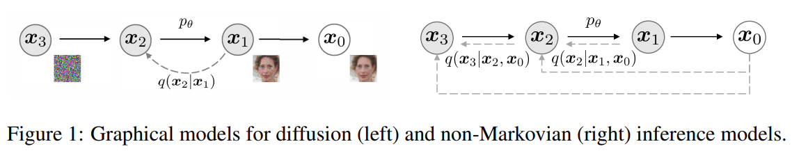
• Section 3: DDPM의 forward diffusion process를 generalize 하여 Markovian Process를 Non-markovian process로 변환하지만, 여전히 reverse markovian chain을 설계할 수 있다.

• Section 4.1: DDPM과 training objective가 동일하므로 (same loss function) 기존과 동일한 신경망을 사용하면서 diffusion process만 non-markovian process로 바꾸기 때문에 많은 generative model에서 자유롭게 신경망을 선택할 수 있다.

• Section 4.2: non-Markovian diffusion process(forward)를 통해 짧은 generative markov chain(reverse)을 형성하여 작은 수의 step으로도 simulation될 수 있도록 한다. 이는 작은 sample quality cost로도 sampling 효율을 크게 늘릴 수 있다.

• Section 5: DDIM이 DDPM에 비해 갖는 장점을 실험을 통해 제시한다.

• 1) Sampling 속도를 10~100배로 가속화해도 DDPM보다 높은 sample generation quality를 갖는다

• 2) DDIM sample들은 "consistency" 특성을 갖는다

동일한 초기 latent variable로 시작하여 다양한 길이의 markov chain으로 여러 sample을 생성하면 sample들이 높은 일관성을 가진다.

• 3) 위의 "consistency" 특성으로 인해 DDIM은 latent variable을 조작하여 meaningful image interpolation이 가능하지만, DDPM은 stochastic generative process로 인해 image space 근처에서 interpolation을 수행해야 한다.

2. Background - DDPM review

DDPM에 대해 보다 더 자세한 내용을 알고 싶다면 아래의 post를 참고하자.

[Paper Review] Denoising Diffusion Probabilistic Model (DDPM)

이번에 리뷰할 논문은 DDPM이라 불리는 Denoising Diffusion Probabilistic Model이다. 해당 Paper는 아래의 링크에서 찾을 수 있다. Denoising Diffusion Probabilistic ModelsWe present high quality image synthesis results using diffusion probabilistic models, a class of latent variable models inspired by considerations from nonequilibrium thermodynamics. Our best results are obtained by training on

Jaewon | Action Precedes MotivationJaewon Kim

Probabilistic Generative Model들의 목적은 다음과 같다.

Real data distribution $\mathbf{x}_0 \sim q(\mathbf{x}_0)$의 sample $\mathbf{x}_0$ 주어졌을 때,

well-known (simple, tractable) distribution $z$ 에서 real data distribution $q(\mathbf{x}_0)$으로 mapping하는 Generative Model를 Training 시킨다.

$q(\mathbf{x}_0) \approx p _{\theta}(\mathbf{x}_0)$

실제 Diffusion Model은 다음과 같이 정의된다.

$$p_\theta(\mathbf{x}_0) = \int p_\theta(\mathbf{x}_{0:T})d\mathbf{x} _{1:T}$$

위의 식에서 $p_\theta(\mathbf{x}_0)$는 $\theta$에 대한 $\mathbf{x}_0$의 likelihood function이다.

Diffusion model parameter $\theta$를 조정해서 이 likelihood를 maximize 시키는 것을 MLE(Maximum Likelihood Estimation)이라 하며, 많은 모델들이 MLE 과정을 통해 학습하게 된다.

이렇듯 likelihood function $p_\theta(\mathbf{x}_0)$를 maximize시키는 parameter $\theta$를 최적화 알고리즘을 통해 찾는 것이 학습의 목표이다.

그런데, likelihood function $p_\theta(\mathbf{x}_0)$를 direct하게 maximize하지 못하기 때문에 indirect하게 variational bound를 설정하여 ELBO를 maximize 한다.

$$p_\theta(\mathbf{x}_0) = \int p_\theta(\mathbf{x}_{0:T})d\mathbf{x} _{1:T}, \qquad \text{where} \quad p_\theta(\mathbf{x}_{0:T}) := p_\theta(\mathbf{x}_T)\prod_{t=1}^T p_\theta^{(t)}(\mathbf{x}_{t-1}|\mathbf{x}_t)$$

왼쪽 $p_\theta(\mathbf{x}_0)$은 Diffusion Model, 오른쪽 $p_\theta(\mathbf{x}_{0:T})$은 Reverse Denoising Process에서의 Joint Distribution


latent variable $\mathbf{x}_0, \mathbf{x}_1, ... , \mathbf{x}_T$ 들은 real image $\mathbf{x}_0$와 동일한 sample space $\mathcal{X}$에 존재한다.

$$\max_\theta \mathbb{E}_{q(\mathbf{x}_0)}[\log p_\theta(\mathbf{x}_0)] \geq \max_\theta \mathbb{E}_{q(\mathbf{x}_0,\mathbf{x}_1,\cdots,\mathbf{x}_T)}[\log p_\theta(\mathbf{x}_{0:T}) - \log q(\mathbf{x}_{1:T}|\mathbf{x}_0)]$$

parameter $\theta$는 위의 variational lower bound를 maximize하도록 학습된다.

DDIM 논문에서는 $\leq$로 나오는데, 찾아보니 arXiv에 개재된 논문에 부등호의 방향이 반대로 나와있는 것 같다. 실제로 수식으로 구현을 해봐도 $\geq$가 맞다.

$$q(\mathbf{x}_{1:T}|\mathbf{x}_0) := \prod_{t=1}^T q(\mathbf{x}_t|\mathbf{x}_{t-1}), \quad q(\mathbf{x}_t|\mathbf{x}_{t-1}) := \mathcal{N}\left(\sqrt{\frac{\alpha_t}{\alpha_{t-1}}}\mathbf{x}_{t-1}, \left(1-\frac{\alpha_t}{\alpha_{t-1}}\right)I\right)$$

$q(\mathbf{x}_{1:T}|\mathbf{x}_0)$는 Forward Diffusion Process에서의 approximate posterior인데, latent variable에 대한 inference distribution이라 한다.

VAE와 같은 전형적인 latent variable model들과 다르게, DDPM은 고정된 fixed inference procedure $q(\mathbf{x}_{1:T}|\mathbf{x}_0)$으로 학습을 진행한다.

또한 감소 수열 $\alpha_{1:T} \in (0, 1]^T$로 매개변수화된 Gaussian transition이 있는 다음의 Markov Chain을 사용했다.

실제 DDPM 논문에서는 $\alpha_t$를 $\bar{\alpha}_t$로 표기함에 유의한다.

• Forward(Inference) Process: $q(\mathbf{x}_{1:T}|\mathbf{x}_0)$ (Approximate posterior)
  • observation $\mathbf{x}_0$에 점진적으로 noise를 더하는 과정
• Generative Process: $p_\theta(\mathbf{x}_{0:T})$ (Joint Distribution)
  • noisy observation $\mathbf{x}_T$에서 점진적으로 denoise를 하여 image를 생성하는 과정
• Reverse Process: $q(\mathbf{x}_{t-1}|\mathbf{x}_{t}) \approx p_\theta^{(t)}(\mathbf{x}_{t-1}|\mathbf{x}_{t})$ (Intractable)

Forward Process에 대해 다음과 같이 변형을 할 수 있다.

$$q(\mathbf{x}_t|\mathbf{x}_0) := \int q(\mathbf{x}_{1:t}|\mathbf{x}_0)d\mathbf{x}_{1:(t-1)} = \mathcal{N}(\mathbf{x}_t; \sqrt{\alpha_t}\mathbf{x}_0, (1-\alpha_t)I)$$

위의 식에 의해 sampling된 $\mathbf{x}_t$는 reparameterization을 통해 아래의 식과 같이 나온다.

$$\mathbf{x}_t = \sqrt{\alpha_t}\mathbf{x}_0 + \sqrt{1-\alpha_t}\epsilon, \quad \epsilon \sim \mathcal{N}(0,I)$$

여기서 $\alpha_T$를 0에 충분히 가깝게 설정하면 임의의 $\mathbf{x}_0$에 대하여 $q(\mathbf{x}_T | \mathbf{x}_0)$는 Standard Gaussian Distribution으로 수렴한다.

$$q(\mathbf{x}_T|\mathbf{x}_0) = \mathcal{N}(\mathbf{x}_T; \sqrt{\alpha_T}\mathbf{x}_0, (1-\alpha_T)I)$$

따라서 $p_\theta(\mathbf{x}_T) := \mathcal{N}(0, I)$ 으로 설명하는 것은 자연스럽다.

모든 conditionals가 trainable mean functions $\mu_\theta(\mathbf{x}_t, t)$와 fixed variance $\Sigma_\theta(\mathbf{x}_t, t) = \sigma_t^2\mathbf{I}$를 갖는 Gaussian으로 모델링되면 다음 식으로 단순화할 수 있다.

$$L_\gamma(\epsilon_\theta) := \sum_{t=1}^T \gamma_t\mathbb{E}_{\mathbf{x}_0\sim q(\mathbf{x}_0),\epsilon_t\sim\mathcal{N}(0,I)}\left[|\epsilon_\theta^{(t)}(\sqrt{\alpha_t}\mathbf{x}_0 + \sqrt{1-\alpha_t}\epsilon_t) - \epsilon_t||_2^2\right], \quad \epsilon_\theta := {\epsilon_\theta^{(t)}}_{t=1}^T$$

• $\epsilon_\theta^{(t)}: \mathcal{X} \rightarrow \mathcal{X} \: (\text{indexed by t})$는 trainable parameter $\theta^{(t)}$를 가지는 함수이다.
• $\gamma := [\gamma_1, ... , \gamma_T]$는 $\alpha_{1:T}$에 의존하는 양의 계수이다.

DDPM과 NCSN은 generation performance를 최대화 하기 위해 $\gamma = 1$로 설정했다.

이미 Trained Model(algorithm1)이라면, 구하고자 하는 이미지인 $\mathbf{x}_0$는 prior $p_\theta(\mathbf{x}_T)$에서 $\mathbf{x}_T$를 sampling하는 것부터 시작하여 generative process를 통해 $\mathbf{x}_{t-1}$를 iterative하게 sampling(algorithm2)한다.

Large $T$ (Long Forward Diffusion process)

Advantages

• reverse process가 Gaussian에 가까워지도록 한다.
• Gaussian conditional distribution으로 이루어진 generative process가 good approximation이 되도록 한다.

Disadvantages

• Sampling process에서 모든 $T$개의 iteration이 순서대로 이루어져야 하므로, sample $\mathbf{x}_0$를 얻기 위해서 다른 Deep Generative Model보다 더 오랜 시간이 걸린다.
• 즉, latency가 중요하고 computation이 제한된 상황에서 task를 수행하는데 있어 impractical하다.

3. Variational Inference for Non-Markovian Forward Process

Generative Model이 inference process의 reverse로 approximate되므로 생성 모델에 필요한 iteration의 수를 줄이기 위해 inference process를 다시 생각해야 한다.

여기서 중요하는 것은 DDPM 목적 함수 $L_\gamma$가 marginals $q_\sigma(\mathbf{x}_{t} | \mathbf{x}_0)$에만 의존하며 Joint Distribution $q_\sigma(\mathbf{x}_{1:T} | \mathbf{x}_0)$에는 직접적으로 의존하지 않는다는 것이다.

이때 같은 marginals에 대해서 수많은 joint distribution이 존재하기 때문에 non-Markovian인 inference process에 대해 새로운 joint distribution을 설정할 수 있으며, 이에 대응되는 새로운 generative process가 필요하다.

또한 이 non-Markovian inference process는 DDPM의 목적 함수와 같은 목적 함수를 가진다는 것을 보일 수 있다.

이때 $\sigma$는 Forward Diffusion Process의 Stochastic한 정도를 나타낸다.

0) 정리하면 DDIM의 Key Contribution은 다음과 같다:

1) DDPM forward process의 Generalized version (same training objective, accelerate sampling)


2) Non-Markovian Process를 통해 10~50x faster sampling than DDPM


3) Deterministic generative process를 통해 implicit model들이 high-quality sample들을 생성

즉 DDIM은 DDPM과 동일한 Training Objective(Algorithm1)을 지니지만, Process(Algorithm2)를 가속화시킨다.

이는 DDPM을 Generalize하여 Non-Markovian Forward Process를 사용하면서도, Reverse Generative Markovian Chain을 이용하여 Sampling을 할 수 있기 때문이다.

1) Non - Markov Forward Process

$$q_\sigma(\mathbf{x}_{1:T}|\mathbf{x}_0) := q_\sigma(\mathbf{x}_T|\mathbf{x}_0) \prod_{t=2}^T q_\sigma(\mathbf{x}_{t-1}|\mathbf{x}_t, \mathbf{x}_0)$$

Forward Process를 구성하는 $q_\sigma(\mathbf{x}_{t-1}|\mathbf{x}_t, \mathbf{x}_0)$항은 다음과 같이 구할 수 있다.

DDIM은 모든 time step $t$에서 DDPM과 동일한 Marginal $q_\sigma(\mathbf{x}_{t}|\mathbf{x}_0)$를 가지는 Non-Markovian Posterior $q_\sigma(\mathbf{x}_{t-1}|\mathbf{x}_t, \mathbf{x}_0)$를 구한다. (by pattern recognition 2.115 formula)

모든 $t > 1$에 대하여


$$q_\sigma(\mathbf{x}_{t-1}|\mathbf{x}_t, \mathbf{x}_0) = \mathcal{N}\left(\sqrt{\alpha_{t-1}}\mathbf{x}_0 + \sqrt{1-\alpha_{t-1}-\sigma_t^2} \cdot \frac{\mathbf{x}_t - \sqrt{\alpha_t}\mathbf{x}_0}{\sqrt{1-\alpha_t}}, \sigma_t^2I\right)$$

$$q_\sigma(\mathbf{x}_{t-1}|\mathbf{x}_{t}, \mathbf{x}_0) = \frac{q_\sigma(\mathbf{x}_{t}|\mathbf{x}_{t-1}, \mathbf{x}_0)q_\sigma(\mathbf{x}_{t-1}|\mathbf{x}_0)}{q_\sigma(\mathbf{x}_{t}|\mathbf{x}_0)}$$

기존의 DDPM에서의 Markovian Forward Process는 $q$, DDIM에서의 Non-Markovian Forward Process는 $q_\sigma$로 표시한다.

2) Generative Process

$$ p_\theta(\mathbf{x}_{0:T}) = p_\theta(\mathbf{x}_T)\prod_{t=1}^T p_\theta^{(t)}(\mathbf{x}_{t-1}|\mathbf{x}_t)$$

Generative Process를 구성하는 $p_\theta^{(t)}(\mathbf{x}_{t-1}|\mathbf{x}_t)$의 항은 다음과 같이 구할 수 있다.

$$p_\theta^{(t)}(\mathbf{x}_{t-1}|\mathbf{x}_t) = \begin{cases} \mathcal{N}(f_\theta^{(t)}(\mathbf{x}_1), \sigma_1^2I) & t=1 \\ q_\sigma(\mathbf{x}_{t-1}|\mathbf{x}_t, f_\theta^{(t)}(\mathbf{x}_t)) & t>1 \end{cases}$$

3) Same Training Objective

위에서 구한 Non-markovian Posterior $q_\sigma(\mathbf{x}_{t-1}|\mathbf{x}_{t}, \mathbf{x}_0)$를 DDPM의 Variational bound에 넣는다.

기존 DDPM의 variational bound에서 바뀌는 부분은 $q$가 $q_\sigma$로 바뀌는 것이 전부이다.

이때, DDIM Variational Bound $J_\sigma(\epsilon_\theta)$를 전개하면서 위의 정리된 Generative Process $p_\theta^{(t)}(\mathbf{x}_{t-1}|\mathbf{x}_t)$를 대입한다.

모든 $\sigma > 0$에 대하여, $J_\sigma = L_\gamma + C$인 $\gamma \in \mathbb{R}_{\geq 0}^T$와 $C \in \mathbb{R}$가 존재한다.

따라서 DDIM은 DDPM과 동일한 Training Objective를 가진다.

4) Faster Sampling

DDIM의 경우, random noise $\sigma_t = 0$으로 설정하여 sampling식 안 2개의 term을 제거하고 deterministic process를 형성한다.

위의 식은 결국 $\mathbf{x}_0$을 예측하고 $\mathbf{x}_t$를 다시 복구하는 형태를 지니는데 예측하는 sample의 time step이 굳이 $t-1$이 아니라 $t-2, t-3, \cdots$가 전부 가능하다.

즉, Sampling Process를 더 가속화시키고 싶다면 위의 식에서 $\mathbf{x}_{t-1}, \sqrt{\alpha_{t-1}}$, 그리고 $\sqrt{1 - \alpha_{t-1} - \sigma_t^2}$안의 $\alpha_{t-1}$까지 3개의 term을 $t-1$아니라 다른 time step으로 바꾸면 된다.

따라서 Forward process를 $x_{1:T}$로 정의하지 않고 부분 집합 $\left \{x_{\tau_1},\cdots,x_{\tau_S}\right \}$로 정의하는 방법을 생각해 볼 수 있다.

3.1) Non-Markovian Forward Process

$$q_\sigma(\mathbf{x}_{1:T}|\mathbf{x}_0) := q_\sigma(\mathbf{x}_T|\mathbf{x}_0) \prod_{t=2}^T q_\sigma(\mathbf{x}_{t-1}|\mathbf{x}_t, \mathbf{x}_0)$$

기존의 DDPM에서의 Markovian Forward Process는 $q$, DDIM에서의 Non-Markovian Forward Process는 $q_\sigma$로, 아래에 $\sigma$를 추가해줘서 차이를 준다.

실수 vector $\sigma \in \mathbb{R}_{\geq 0}^{T}$ 에 대한 inference distribution $q_\sigma(\mathbf{x}_{1:T} | \mathbf{x}_0)$은 다음과 같다.

$$q_\sigma(\mathbf{x}_{1:T}|\mathbf{x}_0) := q_\sigma(\mathbf{x}_T|\mathbf{x}_0) \prod_{t=2}^T q_\sigma(\mathbf{x}_{t-1}|\mathbf{x}_t, \mathbf{x}_0)$$

$$ \text{where} \quad q_\sigma(\mathbf{x}_T|\mathbf{x}_0) = \mathcal{N}(\sqrt{\alpha_t}\mathbf{x}_0, (1-\alpha_t)I)$$

Reparameterization Trick을 사용하여 $\quad q_\sigma(\mathbf{x}_T|\mathbf{x}_0)$를 도출하는 것은 DDPM과 동일하다.

모든 $t > 1$에 대하여


$$q_\sigma(\mathbf{x}_{t-1}|\mathbf{x}_t, \mathbf{x}_0) = \mathcal{N}\left(\sqrt{\alpha_{t-1}}\mathbf{x}_0 + \sqrt{1-\alpha_{t-1}-\sigma_t^2} \cdot \frac{\mathbf{x}_t - \sqrt{\alpha_t}\mathbf{x}_0}{\sqrt{1-\alpha_t}}, \sigma_t^2I\right)$$

왜 $q_\sigma(\mathbf{x}_{t-1}|\mathbf{x}_t, \mathbf{x}_0)$의 식을 저렇게 Setting할까?

이는 DDIM에서 모든 time step $t$에 대하여 DDPM과 동일한 Marginal $q_\sigma(\mathbf{x}_{t}|\mathbf{x}_0)$을 가지는 새로운 Non-markovian process $q_\sigma(\mathbf{x}_t|\mathbf{x}_{t-1}, \mathbf{x}_0) $를 찾고자 하기 때문이다.

$$q_\sigma(\mathbf{x}_{t-1}|\mathbf{x}_{t}, \mathbf{x}_0) = \frac{q_\sigma(\mathbf{x}_{t}|\mathbf{x}_{t-1}, \mathbf{x}_0)q_\sigma(\mathbf{x}_{t-1}|\mathbf{x}_0)}{q_\sigma(\mathbf{x}_{t}|\mathbf{x}_0)}$$


$$q_\sigma(\mathbf{x}_{t}|\mathbf{x}_0) = \mathcal{N}(\sqrt{\alpha_t}\mathbf{x}_0, (1 - \alpha_t)I)$$

이에 대한 증명의 concept을 간단하게 설명하자면:

Marginal Gaussian $\mathcal{p}(\mathbf{x})$와 Conditional Gaussian $\mathcal{p}(\mathbf{y} | \mathbf{x})$가 있을 때 $\mathcal{p}(\mathbf{y})$와 $\mathcal{p}(\mathbf{x} | \mathbf{y})$를 구하는 공식이 있다.

Bishop의 Pattern Recognition 2절 115번 공식을 보면 다음과 같다.

따라서 $\mathbf{x}_0$라는 condition은 항상 given이라 생각하고, Marginal $q(\mathbf{x}_{t} | \mathbf{x}_0)$와 Conditional $q(\mathbf{x}_{t-1} | \mathbf{x}_0, \mathbf{x}_{t})$이 주어졌을 때 Marginal $q(\mathbf{x}_{t-1} | \mathbf{x}_0)$을 구한다고 생각하자.

$$q_\sigma(\mathbf{x}_{t}|\mathbf{x}_0) = \mathcal{N}(\mathbf{x}_{t}; \sqrt{\alpha_t}\mathbf{x}_0, (1 - \alpha_t)I)$$


$$q_\sigma(\mathbf{x}_{t-1}|\mathbf{x}_0) = \mathcal{N}(\mathbf{x}_{t-1}; \sqrt{\alpha_{t-1}}\mathbf{x}_0, (1 - \alpha_{t-1})I)$$


$$q_\sigma(\mathbf{x}_{t-1}|\mathbf{x}_0, \mathbf{x}_t) = \mathcal{N}(\mathbf{x}_{t-1}; \sqrt{\alpha_{t-1}}\mathbf{x}_0 + C \cdot (\mathbf{x}_t - \sqrt{\alpha_t}\mathbf{x}_0), \sigma_t^2\mathbf{I})$$

이후 위 식에 따라 정리하면 $C$의 값이 나오고 임의의 variance $\sigma_t^2$에 대한 Non-markovian posterior를 다음과 같이 정리할 수 있다.

모든 $t > 1$에 대하여


$$q_\sigma(\mathbf{x}_{t-1}|\mathbf{x}_t, \mathbf{x}_0) = \mathcal{N}\left(\sqrt{\alpha_{t-1}}\mathbf{x}_0 + \sqrt{1-\alpha_{t-1}-\sigma_t^2} \cdot \frac{\mathbf{x}_t - \sqrt{\alpha_t}\mathbf{x}_0}{\sqrt{1-\alpha_t}}, \sigma_t^2I\right)$$

따라서 본래의 목적인 동일한 Marginal $q_\sigma(\mathbf{x}_{t}|\mathbf{x}_0)$를 가지는 Non-Markovian Posterior $q_\sigma(\mathbf{x}_{t-1}|\mathbf{x}_t, \mathbf{x}_0)$를 구할 수 있게 되었다.

보다 더 자세한 증명은 아래의 블로그를 참고하자.

Welcome to JunYoung’s blog | DDIM(Denoising Diffusion Implicit Models) 이해하기

Diffusion implicit modeling

DDIM(Denoising Diffusion Implicit Models) 이해하기JunYoung

따라서 Mean Function은 의도한대로 Marginals $q_\sigma(\mathbf{x}_T|\mathbf{x}_0)$ 와 match되는 Joint Distribution $q_\sigma(\mathbf{x}_{t-1}|\mathbf{x}_t, \mathbf{x}_0) $을 새롭게 정의한다.

$$q_\sigma(\mathbf{x}_{1:T}|\mathbf{x}_0) := q_\sigma(\mathbf{x}_T|\mathbf{x}_0) \prod_{t=2}^T q_\sigma(\mathbf{x}_{t-1}|\mathbf{x}_t, \mathbf{x}_0)$$

위의 Non-markovian forward process에 대한 증명은 다음과 같다.

$$q_\sigma(\mathbf{x}_{1:T}|\mathbf{x}_0) = q_\sigma(\mathbf{x}_{1}|\mathbf{x}_0) q_\sigma(\mathbf{x}_{2}|\mathbf{x}_1, \mathbf{x}_0) q_\sigma(\mathbf{x}_{3}|\mathbf{x}_2, \mathbf{x}_0) ... q_\sigma(\mathbf{x}_{T}|\mathbf{x}_{T-1}, \mathbf{x}_0)$$

Bayes' Rule에 의해 Forward Process는 다음과 같이 정리된다.

$$q_\sigma(\mathbf{x}_t|\mathbf{x}_{t-1}, \mathbf{x}_0) = \frac{q_\sigma(\mathbf{x}_{t-1}|\mathbf{x}_t, \mathbf{x}_0)q_\sigma(\mathbf{x}_t|\mathbf{x}_0)}{q_\sigma(\mathbf{x}_{t-1}|\mathbf{x}_0)}$$


$q_\sigma(\mathbf{x}_t|\mathbf{x}_{t-1}, \mathbf{x}_0)$ 또한 Gaussian Distribution 이다.

$$= q_\sigma(\mathbf{x}_{1}|\mathbf{x}_0)\frac{q_\sigma(\mathbf{x}_{1}|\mathbf{x}_2, \mathbf{x}_0)q_\sigma(\mathbf{x}_2|\mathbf{x}_0)}{q_\sigma(\mathbf{x}_{1}|\mathbf{x}_0)} \frac{q_\sigma(\mathbf{x}_{2}|\mathbf{x}_3, \mathbf{x}_0)q_\sigma(\mathbf{x}_3|\mathbf{x}_0)}{q_\sigma(\mathbf{x}_{2}|\mathbf{x}_0)}... \frac{q_\sigma(\mathbf{x}_{T-1}|\mathbf{x}_T, \mathbf{x}_0)q_\sigma(\mathbf{x}_T|\mathbf{x}_0)}{q_\sigma(\mathbf{x}_{T-1}|\mathbf{x}_0)} $$

$$= q_\sigma(\mathbf{x}_T|\mathbf{x}_0) \prod_{t=2}^T q_\sigma(\mathbf{x}_{t-1}|\mathbf{x}_t, \mathbf{x}_0)$$

이 때, $\mathbf{x}_t$가 $\mathbf{x}_{t-1}, \mathbf{x}_0$ 모두에 의존하므로 DDIM의 Forward Process는 더 이상 Markovian이 아니다.

$\sigma$의 크기로 얼마나 Forward Process가 stochastic인지를 조절할 수 있으며, $\sigma \rightarrow 0$일 때 어떤 $t$에 대해 $\mathbf{x}_0, \mathbf{x}_t$를 알면 고정된 $\mathbf{x}_{t-1}$을 알 수 있는 극단적인 경우에 해당한다.

3.2) Generative Process and Unified Variational Inference Objective

$$ p_\theta(\mathbf{x}_{0:T}) = p_\theta(\mathbf{x}_T)\prod_{t=1}^T p_\theta^{(t)}(\mathbf{x}_{t-1}|\mathbf{x}_t)$$

Forward Process만 Non-markov chain이지, Generative Process는 generative markov chain으로 구성되어 있어 DDPM에서의 식과 동일하다.

다음으로 각 $p_\theta^{(t)}(\mathbf{x}_{t-1}|\mathbf{x}_t)$가 $q_\sigma(\mathbf{x}_{t-1}|\mathbf{x}_t, \mathbf{x}_0)$에 대한 지식을 활용하는 학습 가능한 generative process $p_\theta(\mathbf{x}_{0:T})$를 정의한다.

$\mathbf{x}_t$가 주어지면 먼저 대응되는 $\mathbf{x}_0$를 예측하고 이를 이용하여 $q_\sigma(\mathbf{x}_{t-1}|\mathbf{x}_t, \mathbf{x}_0)$로 $\mathbf{x}_{t-1}$을 샘플링한다.

$\mathbf{x}_0 \sim q(\mathbf{x}_0)$와 $\epsilon_t \sim \mathcal{N}(0, I)$에 대하여 $\mathbf{x}_t = \sqrt{\alpha_t}\mathbf{x}_0 + \sqrt{1-\alpha_t}\epsilon_t$로 계산할 수 있다.

그 다음 모델 $\epsilon_\theta^{(t)}(\mathbf{x}_t)$가 $\mathbf{x}_0$에 대한 정보 없이 $\mathbf{x}_t$로부터 $\epsilon_t$를 예측한다.

식을 다음과 같이 다시 세우면 주어진 $\mathbf{x}_t$에 대한 $\mathbf{x}_0$의 예측인 denoised observation을 얻을 수 있다.

$$f_\theta^{(t)}(\mathbf{x}_t) := \frac{1}{\sqrt{\alpha_t}}(\mathbf{x}_t - \sqrt{1-\alpha_t}\epsilon_\theta^{(t)})$$

그런 다음 고정된 prior $p_\theta(\mathbf{x}_T) = \mathcal{N}(0,I)$에 대한 generative process를 다음과 같이 정의할 수 있다.

$$p_\theta^{(t)}(\mathbf{x}_{t-1}|\mathbf{x}_t) = \begin{cases} \mathcal{N}(f_\theta^{(t)}(\mathbf{x}_1), \sigma_1^2I) & t=1 \\ q_\sigma(\mathbf{x}_{t-1}|\mathbf{x}_t, f_\theta^{(t)}(\mathbf{x}_t)) & t>1 \end{cases}$$

$q_\sigma(\mathbf{x}_{t-1}|\mathbf{x}_t, f_\theta^{(t)}(\mathbf{x}_t))$는 위에서 정의한 $q_\sigma(\mathbf{x}_{t-1}|\mathbf{x}_t, \mathbf{x}_0)$ 식에 $\mathbf{x}_0$ 대신 $f_\theta^{(t)}(\mathbf{x}_t)$를 대입하여 정의할 수 있다.

Generative process가 모든 $t$에서 설명하도록 $t = 1$인 경우에 약간의 Gaussian noise를 추가한다.

파라미터 $\theta$는 다음 목적 함수로 최적화된다.

기존의 DDPM의 Variational bound에서의 Markovian process $q$가 DDIM에서는 Non-Markovian process로 $q_\sigma$로 변환된 부분을 제외하면 전부 동일하다.

$$J_\sigma(\epsilon_\theta) := \mathbb{E}_{\mathbf{x}_{0:T}\sim q_\sigma(\mathbf{x}_{0:T})}[\log q_\sigma(\mathbf{x}_{1:T}|\mathbf{x}_0) - \log p_\theta(\mathbf{x}_{0:T})]$$

앞 항에 Forward Process, 뒷 항에 Generative Process의 식을 넣어준다.

$$= \mathbb{E}_{\mathbf{x}_{0:T}\sim q_\sigma(\mathbf{x}_{0:T})}\left[\log\left(q_\sigma(\mathbf{x}_T|\mathbf{x}_0)\prod_{t=2}^T q_\sigma(\mathbf{x}_{t-1}|\mathbf{x}_t, \mathbf{x}_0)\right) - \log\left(p_\theta(\mathbf{x}_T)\prod_{t=1}^T p_\theta^{(t)}(\mathbf{x}_{t-1}|\mathbf{x}_t)\right)\right]$$

$$= \mathbb{E}_{\mathbf{x}_{0:T}\sim q_\sigma(\mathbf{x}_{0:T})}\left[\log q_\sigma(\mathbf{x}_T|\mathbf{x}_0) + \sum_{t=2}^T \log q_\sigma(\mathbf{x}_{t-1}|\mathbf{x}_t, \mathbf{x}_0) - \sum_{t=1}^T \log p_\theta^{(t)}(\mathbf{x}_{t-1}|\mathbf{x}_t) - \log p_\theta(\mathbf{x}_T)\right]$$

$J_\sigma$의 정의를 보면 $\sigma$에 따라 목적 함수가 다르기 때문에 다른 모델이 필요하다는 것을 알 수 있다.

즉, 다음이 성립한다.

모든 $\sigma > 0$에 대하여, $J_\sigma = L_\gamma + C$인 $\gamma \in \mathbb{R}_{\geq 0}^T$와 $C \in \mathbb{R}$가 존재한다.

이에 대한 증명은 다음과 같다.

Variational objective $L_\gamma$의 특별한 점은 Model $\epsilon_\theta^{(t)}$의 parameter가 다른 $t$에 공유되지 않는 경우 $\epsilon_\theta^{(t)}$에 대한 최적해가 가중치 $\gamma$에 의존하지 않는다는 것이다.

Variational objective $L_\gamma$의 특별한 점은 Model $\epsilon_\theta^{(t)}$의 parameter가 다른 $t$에 공유되지 않는 경우 $\epsilon_\theta^{(t)}$에 대한 최적해가 가중치 $\gamma$에 의존하지 않는다는 것이다.

위의 phrase가 어떠한 뜻인지 해석이 안된다. 나중에 찾아볼 것!

이러한 성질은 두 가지 의미를 갖는다.

• DDPM의 variational lower bound에 대한 목적 함수로 $L_1$을 사용하는 것이 가능하다.

• $J_\sigma$가 일부 $L_\gamma$와 같이 때문에 $J_\sigma$의 최적해는 $L_1$의 해와 동일하다.

즉 $\epsilon_\theta^{(t)}$가 다른 $t$에 공유되지 않는 경우 DDPM에서의 objective $L_1$을 DDIM에서의 variational objective $J_\sigma$로 대체해서 사용가능하다.

4. Sampling from Generalized Generative Processes

Markovian forward process를 위한 generative process (DDPM)뿐만 아니라 non-Markovian forward process를 위한 generative process(DDIM)도 $L_1$을 학습할 수 있다.

따라서 pre-trained DDPM을 new objective에 대한 solution으로 사용할 수 있으며 $\sigma$를 변경하여 필요에 따라 샘플을 더 잘 생성하는 generative process를 찾는 데 집중할 수 있다.

즉, 어차피 DDPM과 DDIM의 경우 Training Objective가 $L_1$으로 동일하고 Sampling Process를 가속화한 것이므로, Training(Algorithm1)은 Pre-trained DDPM을 이용하고 Sampling(Algorithm2)은 DDIM으로 하는 것이 효율적이다.

4.1) Denoising Diffusion Implicit Models

다음 식으로 $x_t$로부터 $x_{t-1}$을 생성할 수 있다.

$\epsilon_t \sim \mathcal{N}(0,I)$는 $x_t$에 독립적인 가우시안 noise이며, $\alpha_0 := 1$로 정의한다.

$\sigma$를 변경하면 같은 모델 $\epsilon_\theta$를 사용하여도 generative process가 달라지기 때문에 모델을 다시 학습하지 않아도 된다.

이때 $\sigma$는 Forward Diffusion Process의 Stochastic한 정도를 나타낸다.

모든 $t$에 대하여

$$\sigma_t = \sqrt{\frac{1-\alpha_{t-1}}{1-\alpha_t}}\sqrt{1 - \frac{\alpha_t}{\alpha_{t-1}}}$$

로 두면 forward process가 Markovian이 되며 generative process가 DDPM이 된다.

모든 $t$에 대하여 $\sigma_t = 0$으로 두면, 주어진 $x_{t-1}$와 $x_0$에 대하여 forward process가 deterministic해진다. (단, $t=1$일 때는 제외)

Generative Process에서는 random noise $\epsilon_t$ 앞의 계수 $\sigma_t=0$이 된다.

이 경우 $x_T$부터 $x_0$까지 모두 고정되어 샘플링되기 때문에 모델이 implicit probabilistic model이 된다.

이를 DDPM 목적 함수로 학습된 implicit probabilistic model이기 때문에 Denoising Diffusion Implicit Model (DDIM)이라 부른다.

4.2) Accelerated Generation Processes

DDPM의 경우 forward process가 $T$ step으로 고정되어 있기 때문에 generative process도 $T$ step으로 강제된다.

반면 $L_1$은 $q_\sigma(x_t|x_0)$가 고정되어 있는 한 특정 forward 방식에 의존하지 않으므로 T보다 작은 길이의 forward process를도 고려할 수 있다.

위의 식을 자세히 보면,

Prediction과 Direction은 $\epsilon_\theta^{(t)}(\mathbf{x}_t)$라는 Model이 예측된 noise를 기반으로 한다.

1) $\mathbf{x}_t$가 given

2) $\mathbf{x}_0$를 predict: 현재 상태($\mathbf{x}_{t}$)에서 다음 상태 ($ \mathbf{x}_{t-1}$)로 이동할 때, 예측된 원본 이미지 $\mathbf{x}_{t}$를 기반으로 한다.

3) direction pointing to $\mathbf{x}_t$: 현재 상태($\mathbf{x}_{t}$) 로부터 noise를 제거하는 방향을 나타낸다.

4) random noise: DDPM과 동일하게 각 time step 마다 추가되는 standard gaussian noise이고, 각 sampling process에서 stochastic 특성을 추가하여 모델의 유연성을 확보한다.

DDIM의 경우, random noise $\sigma_t = 0$으로 설정하여 sampling식 안 2개의 term을 제거하고 deterministic process를 형성한다.

위의 식은 결국 $\mathbf{x}_0$을 예측하고 $\mathbf{x}_t$를 다시 복구하는 형태를 지니는데 예측하는 sample의 time step이 굳이 $t-1$이 아니라 $t-2, t-3, \cdots$가 전부 가능하다.

즉, Sampling Process를 더 가속화시키고 싶다면 위의 식에서 $\mathbf{x}_{t-1}, \sqrt{\alpha_{t-1}}$, 그리고 $\sqrt{1 - \alpha_{t-1} - \sigma_t^2}$안의 $\alpha_{t-1}$까지 3개의 term을 $t-1$아니라 다른 time step으로 바꾸면 된다.

따라서 Forward process를 $x_{1:T}$로 정의하지 않고 부분 집합 $\left \{x_{\tau_1},\cdots,x_{\tau_S}\right \}$로 정의하는 방법을 생각해 볼 수 있다.

여기서 $\tau$는 길이가 $S$인 $[1,\cdots,T]$의 부분 집합이다. ($T$ 중에서 $S$만큼 선택)


특히 $q(\mathbf{x}_{\tau_i} | \mathbf{x}_0) = \mathcal{N}(\sqrt{\alpha_{\tau_i}}x_0, (1-\alpha_{\tau_i})I)$가 주어졌을 때 $x_{\tau_1},\cdots,x_{\tau_S}$에 대한 forward process를 정의한다.

그러면 generative process도 reversed $\tau$에 따라 latent variable을 샘플링하며 이를 샘플링 궤적(trajectory)이라 한다.

샘플링 횟수의 길이가 $T$보다 짧아지면 샘플링 과정의 computational efficiency가 상당히 증가한다.

정리하면 DDIM도 마찬가지로 $L_1$ Loss를 이용해 훈련하기에 training에 어떠한 change도 필요 없다.

이는 우리가 임의의 숫자의 forward process으로 training시킬 수 있으나 이 중 일부만 generative process에서 sampling된다는 문제가 있다.

4.3) Relevance to Neural ODEs

DDIM 샘플링 식($\sigma_t = 0$)을 다음과 같이 다시 쓸 수 있으며, 상미분방정식(ODE)를 풀기 위한 Euler intergration과 비슷해진다.

$$x_{t-\Delta t} = \sqrt{\alpha_{t-\Delta t}}\left(\frac{x_t - \sqrt{1-\alpha_t}\epsilon_\theta^{(t)}(x_t)}{\sqrt{\alpha_t}}\right) + \sqrt{1-\alpha_{t-\Delta t}} \cdot \epsilon_\theta^{(t)}(x_t)$$

$$= \frac{\sqrt{\alpha_{t-\Delta t}}}{\sqrt{\alpha_t}}x_t + \sqrt{\alpha_{t-\Delta t}}\left(\sqrt{\frac{1-\alpha_{t-\Delta t}}{\alpha_{t-\Delta t}}} - \sqrt{\frac{1-\alpha_t}{\alpha_t}}\right) \cdot \epsilon_\theta^{(t)}(x_t)$$

$$\frac{x_{t-\Delta t}}{\sqrt{\alpha_{t-\Delta t}}} = \frac{x_t}{\sqrt{\alpha_t}} + \left(\sqrt{\frac{1-\alpha_{t-\Delta t}}{\alpha_{t-\Delta t}}} - \sqrt{\frac{1-\alpha_t}{\alpha_t}}\right)\epsilon_\theta^{(t)}(x_t)$$

$\sqrt{(1-\alpha)/\alpha} = \sigma, x/\sqrt{\alpha} = \bar{x}$로 치환하면 ODE를 구할 수 있다.

$$\bar{x}_{t-\Delta t} = \bar{x}_t + (\sigma_{t-\Delta t} - \sigma_t)\epsilon_\theta^{(t)}(x_t)$$

$$\bar{x}_t - \bar{x}_{t-\Delta t} = (\sigma_t - \sigma_{t-\Delta t})\epsilon_\theta^{(t)}\left(\frac{\bar{x}_t}{\sqrt{1+\sigma_t^2}}\right)$$

$$\therefore d\bar{x}(t) = \epsilon_\theta^{(t)}\left(\frac{\bar{x}(t)}{\sqrt{\sigma^2+1}}\right)d\sigma(t)$$

초기 조건은 $x(T) \sim \mathcal{N}(0,\sigma(T))$이다.

이를 통해 알 수 있는 것은 충분한 discretization steps을 거치면 ODE를 reverse해서 generation process의 reverse, 즉 encoding $(x_0 \rightarrow x_T)$도 가능하다는 것이다.

Probability flow ODE에서는 SDE(Stochastic Differential Equation)의 Marginal Density를 구하고자 하는데, 이때 동일한 sampling schedule을 적용할 수 있다.

여기서 Proposition 1을 적용할 수 있다:

$$d\bar{x}(t) = \epsilon_\theta^{(t)}\left(\frac{\bar{x}(t)}{\sqrt{\sigma^2+1}}\right)d\sigma(t)$$

위의 Neural ODE의 optimal model $\epsilon_\theta^{(t)}$은 Variance-Exploding SDE에 대응되는 Probability flow ODE와 동일하다.

다만 ODE가 동일하다고 해도, Probability flow ODE에 적용되는 Euler method가 가 다음과 같이 update하므로 sampling procedure가 다르다.

• Neural ODE: $$\frac{x_{t-\Delta t}}{\sqrt{\alpha_{t-\Delta t}}} = \frac{x_t}{\sqrt{\alpha_t}} + \left(\sqrt{\frac{1-\alpha_{t-\Delta t}}{\alpha_{t-\Delta t}}} - \sqrt{\frac{1-\alpha_t}{\alpha_t}}\right)\epsilon_\theta^{(t)}(x_t)$$

• Probability Flow ODE: $$\frac{x_{t-\Delta t}}{\sqrt{\alpha_{t-\Delta t}}} = \frac{x_t}{\sqrt{\alpha_t}} + \frac{1}{2}\left(\frac{1-\alpha_{t-\Delta t}}{\alpha_{t-\Delta t}} - \frac{1-\alpha_t}{\alpha_t}\right) \cdot \sqrt{\frac{\alpha_t}{1-\alpha_t}} \cdot \epsilon_\theta^{(t)}(x_t)$$

두 식은 $\alpha_t$와 $\alpha_{t-\Delta t}$가 비슷할 경우 동일해진다.

다만 DDIM과 같이 fewer sampling step에서는 차이를 만든다.

Neural ODE의 경우 $d\sigma(t)$에 의존하지만 Probability Flow ODE는 $dt$에 의존하여 Euler Step를 사용한다.

5. Experiments

저자들은 DDIM에 대해 다음의 3가지 결과를 보여준다:

1) DDIM outperform DDPM: Image Generation @ fewer iterations

• speed up 10x ~ 100x over DDPM generation process

2) initial random variable $\mathbf{x}_T$가 fix되면 DDPM과 달리 generation trajectory와 상관없이 DDIM은 high-level image feature들을 보유하게 된다.

• interpolation을 direct하게 구현할 수 있다.

3) latent code로부터 reconstruct하여 sample들을 encode할 수 있다.

• DDIM의 deterministic generative process에 의해 가능하다.

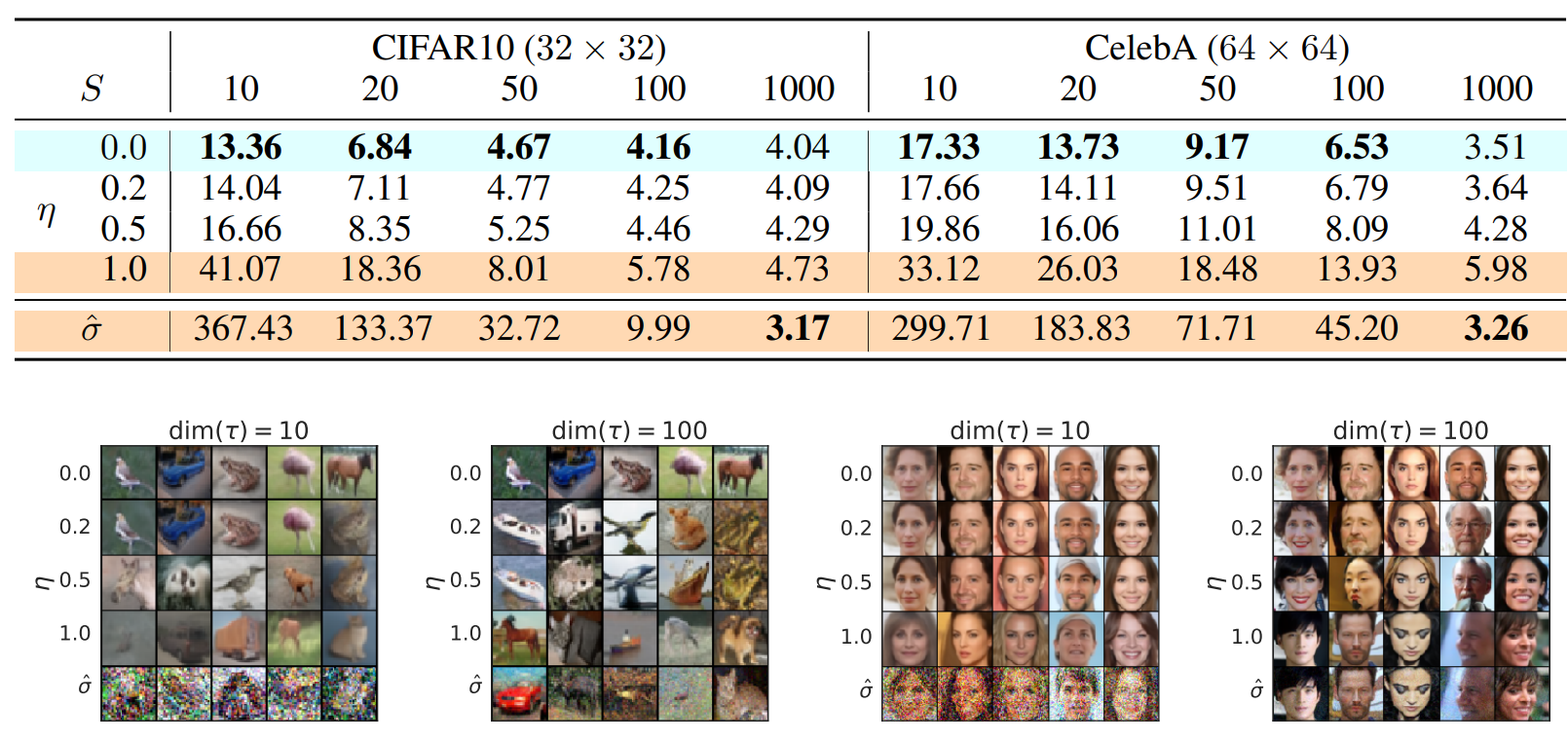
• DDPM과 같은 모델을 같은 목적 함수로 $T = 1000$에 대하여 학습
• Training procedure은 동일, Sampling method를 변화

• $τ$와 $\sigma$를 조절해가면 실험 진행
  • $τ$: controls how fast the samples are obtained
• $\sigma$: interpolates b/w the deterministic DDIM and the stochastic DDPM

쉬운 비교를 위해 $\sigma$를 다음과 같이 정의

$$\sigma_\tau(\eta) = \eta\sqrt{\frac{1-\alpha_{\tau_{i-1}}}{1-\alpha_{\tau_i}}}\sqrt{1-\frac{\alpha_{\tau_i}}{\alpha_{\tau_{i-1}}}}$$

$\eta = 0$이면 DDIM이고 $\eta = 1$이면 DDPM이다.

또한 표준편차가

$$\hat{\sigma}_{\tau_i} = \sqrt{1-\frac{\alpha_{\tau_i}}{\alpha_{\tau_{i-1}}}}$$

인 DDPM에 대하여도 실험하였으며,

이는 random noise가 $\sigma(1)$보다 더 큰 표준편차를 갖는 경우이다.

다만 이 standard deviation $\hat{\sigma}_{\tau_i}$을 사용하는 경우는 오직 CIFAR10 Sample을 얻는 경우에만 해당한다.