[Paper Review] CTGAN: Modeling Tabular Data using Conditional GAN
![[Paper Review] CTGAN: Modeling Tabular Data using Conditional GAN](/content/images/size/w1200/2024/07/-----2024-07-21-073107.png)
해당 논문은 Tabular Data를 생성하는 CTGAN, TVAE 모델에 대해 설명한다.
논문의 arXiv Link는 다음과 같다.
참고한 자료는 아래와 같다.
 dong1
dong1 미슈니
미슈니
 dororo_27
0. Abstract
Tabular Data의 row의 probability distribution을 modeling하는 것과 realistic synthetic data를 생성하는 것은 쉽지 않은 일이다.
Tabular Data는 주로 discrete하거나 continuous column들로 구성되어 있다.
- Continuous: multiple node를 가지고 있음
- Discrete: imbalance가 modeling을 힘들게 함
논문의 저자들은 CTGAN을 제안하여, 모델의 conditional generator가 이러한 문제를 해결하도록 했다.
공정한 성능의 평가를 위해 여러 개의 real dataset과 bayesian network basline들을 이용하여 benchmark 시스템을 제안했고, CTGAN이 여러 Bayesian method들을 압도하는 결과를 보여준다.
1. Introduction
최근 Deep Generative Model들이 활발히 연구되면서, Probability Distribution을 더 정교하고 정확하게 예측하는 좋은 성능의 생성 모델들이 나오고 있다.
이러한 상황속에서, Generative Model들의 성능을 evaluate할 수 있는 benchmarking system은 중요하게 작용한다.
3개의 recent technique(MedGAN, VeeGAN, TableGAN)들을 implement하고, 이들을 baseline method인 2개의 Bayesian Network(CLBN, PrivBN)들과 비교했다.

아쉽게도, 위의 recent technique들은 likelihood fitness나 machine learning efficacy등의 evaluation metric에 대해 baseline method들에 비해 성능이 좋지 않았다.
이는 아래의 GAN이 가지고 있는 아래의 challenge들을 이유로 들 수 있다.
- Discrete and Continuous Column들을
동시에 Modeling해야하는 문제 - Continuous Column에 있는
multi-modal non-Gaussian value들의 문제- 확률 분포가 여러 개의 봉우리를 가지게 되는 성질
- Categorical(Discrete) Column에 있는
severe imbalance문제- 각 category별로 빈도수가 모두 다르다는 성질
따라서 저자들은 Conditional Tabular GAN(CTGAN)을 제안했고, 이는 다음의 새로운 technique들을 소개한다.
- Training Procedure: augmentation with
mode-specific normalization - Architectural Changes
- Data Imbalance:
Conditional Generator와train-by-sampling으로 해결
위의 Table 1에서 볼 수 있듯이, CTGAN은 다른 Baeysian Network baseline과 다른 GAN Model들에 비해 매우 높은 성능을 보여주었다.
CTGAN의 Main Contribution은 아래의 2가지로 설명할 수 있다.
1) Conditional GANs for synthetic data generation
CTGAN을 synthetic tabular data generator로 사용할 경우 적어도 87.5%의 dataset에서 outperform을 할 뿐만 아니라 새롭게 제시한 TVAE Model도 3개의 dataset에서 outperform한다.2) A benchmarking system for synthetic data generation algorithms
저자들은comprehensive benchmark framework를 design했다.
open source이기에, 다른 method나 additional dataset을 추가할 수 있다. 논문을 쓴 시점에는 5개의 DL Model과, 2 Bayesian Network Model, 15 Datasets, 2 evaluation metric이 존재한다.
2. Related Work
기존에 synthetic data의 생성은 각 column들을 random variable로 취급하여 joint multivariate distribution을 modeling하고, 해당 분포에서 sampling 하여 이루어진다고 보았다.
- Decision Tree, Bayesian Networks, Copulas 등이 이에 해당한다.
다만 이러한 모델들은 distribution의 type에 크게 영향을 받고, computational issue들에 의해 synthetic data의 fidelity를 limit한다.
Generative Model들이 발전하고 확장되면서, tabular data의 생성에도 주로 사용되었다. medGAN, ehrGAN, tableGAN, PATE-GAN 등이 그 예시이다.
3. Challenges with GANs in Tabular Data Generation Task
Synthetic Data Generation을 위해 아래의 사항들이 필요하다:
- $G$: Data Synthesizer
- $\mathbf{T}$: (Real) Ground Table
- $N_c$: Continuous Column의 개수 ($\left\{C_1, C_2, ... , C_{N_c}\right\}$)
- $N_d$: Discrete Column의 개수 ($\left\{D_1, D_2, ... , D_{N_d}\right\}$)
- $\mathbf{T}_{\text{syn}}$: (Generated) Synthetic Table
Tabular Data Size: $n \times (N_c + N_d)$
각 column들은 Random Variable로 취급하고, $\mathbb{P}\left(C_{1:N_c}, D_{1:N_d}\right)$라는unknown joint distribution을 따른다.
Total Column 개수: $N_c + N_d$
Total Row 개수: $n$
$j$번째 Row $\mathbf{r}_j = \left\{c _{1, j}, ... , c _{N_c, j}, d_{1, j}, ... , d_{N_d, j} \right\}, j \in \left\{1, ... , n\right\}$
실제 Ground Table인 $\mathbf{T}$는 Training Set $\mathbf{T}_{\text{train}}$과 Test Set $\mathbf{T}_{\text{test}}$로 나뉜다.
Data Synthesizer $G$를 $\mathbf{T}_{\text{train}}$에 대해 훈련시킨 후, 생성된 $\mathbf{T}_{\text{syn}}$는 $G$에서 independently하게 각 row들을 sampling하여 생성한다.
이렇게 생성된 $\mathbf{T}_{\text{syn}}$, 즉 Data Synthesizer $G$의 성능은 2개의 metric으로 평가된다.
1) Likelihood Fitness
Generated $\mathbf{T}_{\text{syn}}$가 Ground Train $\mathbf{T}_{\text{train}}$와 같은 joint distribution을 따르는가?
2) Machine Learning Efficacy
$\mathbf{T}_{\text{train}}$를 학습하여 생성된 $\mathbf{T}_{\text{syn}}$를 이용하여 Train한 Classifier나 Regressor의 성능과,
$\mathbf{T}_{\text{test}}$를 이용하여 Train한 Classifier나 Regressor의 성능이 얼마나 비슷한가?

이러한 Metric이 좋은 성능을 내기 위해서는 아래의 Challenge들을 해결해야 한다:
Mixed Data Types (1)
Discrete, Continous Column들의 mix를 생성해야 하므로, GAN은 softmax(discrete)와 tanh(continuous) activation을 각각 output에 적용해야 한다.
Non-Gaussian Distributions (2)
Generator의 output layer에는 주로 $[-1, 1]$으로 Normalized된 Image pixel(followgaussian-like distribution)을 생성하기 위해 tanh가 들어간다.
다만 Tabular data의 continuous column들은non-gaussian을 주로 따르기에 min-max normalization은 gradient vanishing problem을 일으킬 가능성이 크다.
Multimodal Distributions (3)
KDE(kernel density estimation)을 이용하여 column안에 있는 mode의 개수를 예측한다.
Vanilla GAN은 간단한 2D Dataset에 있는 모든 mode들을 다 예측할 수 없는 문제점을 가진다. 이는 continuous column의 multimodal distribution을 modeling 하기 힘들도록 한다.
Learning form space one-hot-encoded vectors (4)
synthetic sample을 생성할 때, Generative Model은 모든 category(discrete)의 probability distribution을 구하기 위해softmax함수를 사용하지만, real-data는one-hot vector로 이루어져 있다.
이는 GAN의 Discriminator가 실제 row의 realness를 평가하는 것이 아니라, distribution의 sparseness를 보고 평가할 수 있어 문제가 된다.
Highly imbalanced categorical columns (5)
categorical(discrete) column들은 매우 높은 확률로 imbalanced 되는 경우가 많다. 즉, major category가 90% 이상 등장하는 경우가 많다는 것이다.
이는 severe mode가 붕괴되도록 하고, minor category를 놓치는 경우 discriminator가 발견하기 힘든 작은 변화가 distribution에 일어난다.
또한 minor class에 대한 insufficient training opportunities를 제공한다.
4. CTGAN Model
CTGAN Model은 GAN-based tabular data distribution을 modeling하는 방법론이고, 해당 distribution에서 sampling하여 tabular data를 생성한다.
CTGAN에서는 Mode-Specific Normalization을 수행하여 Non-Gaussian$(2)$ 과 Multimodal Distribution$(3)$ 을 극복하도록 하고,
Conditional Generator를 design하고, Training-by-Sampling을 통해 imbalanced discrete column$(5)$ 들을 다룬다.
이후 FC-Layer와 several technique들을 사용하여 high-quality model들을 훈련할 수 있도록 한다.
4.1) Notations
CTGAN Paper에서는 아래와 같이 Notation들을 정의했다.
- $x_1 \oplus x_2 \oplus \ldots$: This denotes
concatenationof vectors $x_1, x_2, \ldots$
- $\text{gumbel}_\tau(x)$: This applies
Gumbel softmaxwith parameter $\tau$ on a vector $x$.
- $\text{leaky}_\gamma(x)$: This applies a
leaky ReLUactivation on $x$ with leaky ratio $\gamma$.
- $\text{FC}_{u \to v}(x)$: This applies a
linear transformationon a $u$-dimensional input to get a $v$-dimensional output.
4.2) Mode-specific Normalization
Tabular Data를 생성하기 전에 Normalization 과정을 거쳐야 한다.
Discrete value들은 Category 개수만큼 one-hot vector로 간단하게 나타낼 수 있는 것과 달리, arbitrary distribution을 가지고 있는 continuous value들은 나타내는 방법이 중요하다.
이전의 GAN 모델들이 $[-1, 1]$의 범위로 continuous value들을 normalize시키기 위해 min-max normalization을 사용했다.
CTGAN에서는 mode-specific normalization을 이용하여 complicated distribution을 가지는 continuous column들을 다루려고 한다.
아래의 문제들을 Mode-specific Normalization들을 활용하여 해결한다.- Non-Gaussian Distribution
- Multimodal Distributions
Mode-specific Normalization은 각 column을 독립적으로 처리하며, 3단계의 과정을 따른다.
일반적으로 Continuous Data를 가지는 하나의 column의 경우, 해당 column의 distribution은 여러 개의 gaussian이 결합한 Gaussian Mixture의 분포를 따른다.

이러할 경우 제대로 데이터를 생성하기 어렵기 때문에 Normalization 과정을 거쳐야 한다.
우선 결합한 Gaussian의 개수만큼의 Sub-Gaussian Distribution으로 분해해야 한다.
1) 각 $i$번째 Continuous Column $C_i$마다 VGM(Variational Gaussian Model)을 사용하여 mode의 개수 $m_i$를 예측하고 mode의 개수만큼 Sub-Gaussian Mixture에 fitting한다. (각 Mode의 $\mu_k, \phi_k$를 구한다)
예를 들어, 아래의 그림에는 VGM가 3개의 mode를 찾는다. ($m=3, \eta_1, \eta_2, \eta_3$라 하자.)

학습된 Gaussian Mixture Model은 다음과 같다.
$$P(C_{i,j}) = \sum_{k=1}^{m_i} \mu_k \mathcal{N}(C_{i,j}; \eta_k, \phi_k)$$
$\mu_k, \phi_k$: weight, standard deviation of a mode
즉, VGM을 이용하여 여러 개의 Sub-Gaussian Distribution으로 분해 후, 각 Sub distribution의 $\mu_k, \phi_k$ (weight, standard deviation)을 미리 구해둔다.
2) $i$번째 continuous column $C_i$의 각 $j$번째 원소 (jth row) $c_{i, j}$에 대해, PDF에 찍어보고 가장 확률이 높게 나오는 Mode(Sub-Gaussian Distribution)을 구한다.
$c_{i, j}$를 각 PDF(sub-distribution)에 찍었을 때 나타나는 y값(probability density)을 $\rho_k$라 하면 다음의 식이 성립한다.
$$\rho_k = \mu_k \mathcal{N}(C_{i,j}; \eta_k, \phi_k)$$
3) 가장 Probability Density가 높게 나오는 Mode $m_i$를 선택하고, 이를 one-hot encoded vector $\beta_{i,j}$로 표시한다.
그리고, $c_{i, j}$에 대응되는 probability value를 $\alpha_{i, j}$라고 할 때 아래의 식을 통해 구할 수 있다.
$$\alpha_{i,j} = \frac{C_{i,j} - \eta_3}{4\phi_3}$$
$$\beta_{i,j} = [0, 0, 1]$$
그럼 이제 최종적으로 각 row별로 Mode-Specific Normalization을 수행하면 된다.
각 Row는 Continuous data와 Discrete한 data가 합쳐져 있으므로 다음의 식을 따라 Concatenate해준다.
$$\mathbf{r}_j = \alpha_{1,j} \oplus \beta_{1,j} \oplus \ldots \oplus \alpha_{N_c,j} \oplus \beta_{N_c,j} \oplus \mathbf{d}_{1,j} \oplus \ldots \oplus \mathbf{d}_{N_d,j}$$
이때, $\mathbf{d}_{1,j}$는 discrete value의 one-hot representation이다.
4.3) Conditional Generator and Training-by-Sampling
아래의 문제들을Conditional GeneratorandTraining-by-Sampling들을 활용하여 해결한다.
- imbalanced discrete columns
이제 normalization 도 마쳤으니, 본격적으로 GAN 학습을 해볼 것이다.
일반적으로 GAN의 Generator는 Multivariate Gaussian Distribution(MVN)에서 sampling된 vector를 입력으로 받아, 이를 data의 distribution으로 mapping 해주는 역할을 한다.
그러나 이러한 training 방법은 categorical column에 있는 data의 빈도수를 고려하지 못하는, class imbalance 문제가 발생한다.
즉 만약 training data가 random하게 training step 도중 random하게 sampling될 경우, minor category의 data는 빈도수에 맞게 training 과정에 반영되지 않을 것이다.
이는 Generator가 real data distribution을 학습하지 못하고, resample된 distribution을 학습하기 때문이다.
따라서 efficient하게 resample하는 방법은 categorical data들이 training process에서 evenly sample(분포와 동일하게) 되어 학습 후,
test process에서 real distribution으로 mapping하는 것이다. (uniformly 라는 말이 아니다)
이는 Conditional Generator를 사용하여 해결할 수 있다.
Conditional Generator는 특정 discrete column$D_{i*}$의 particular value $k^{*}$가 주어졌을 때 row의 conditional distribution을 학습한다.
$$\hat{\mathbf{r}} \sim \mathbb{P}_G(\text{row}|D_{i*} = k^{*})$$
- $k^{*}$:
category(class label)from $i^{*}$th discrete column $D_{i*}$- $k^{*}$, $D_{i*}$는
specific condition$D_{i*} = k^{*}$의 구성요소로특정 값으로 취급한다. (ex: $D_2 = 1$ - $k^{*}$를 각 element로 취급하지 말고,
class label로 취급한다.
- $k^{*}$, $D_{i*}$는
- $\hat{\mathbf{r}}$: generated samples
GAN안에 Conditional Generator를 integrate하는 것은 아래 3개의 사항들을 요구한다:
1) condition과 input을 어떻게 represent할 건지
2) generated row들이 condition을 어떻게 preserve할 건지
3) Conditional Generator가 real data conditional distribution을 어떻게 학습할건지
$$\mathbb{P}_G(\text{row}|D_{i*} = k^{*}) = \mathbb{P}(\text{row}|D_{i*} = k^{*})$$
- $\mathbb{P}(\text{row}|D_{i*} = k^{*})$: $D_{i*}$의 Discrete Column이 $K^{*}$라는 category를 가질 때, 해당 row의 element도 동일한 class를 가질 확률
따라서 우리는 row의 original distribution을 다음의 식을 통해 구할 수 있다:
$$\mathbb{P}(\text{row}) = \sum_{k \in D_{i*}} \mathbb{P}_G(\text{row}|D_{i*} = k^{*})\mathbb{P}(D_{i*} = k)$$
위의 문제들을 해결할 수 있는 3개의 key - elements들을 Conditional Vector, Generator Loss, Training - by - Samling 라 한다.
주어진 condition $D_{i*} = k^{*}$을 mask vector $\mathbf{m}_i$로 처리한다.
- $D_{i*} = k^{*}$: $i^{*}$th discrete column $D_{i*}$이 $ k^{*}$라는 category을 갖는 condition
- $\mathbf{m}_i$라는 mask(one-hot) vector의 $\mathbf{m}_i^{(k)}$ element가 총 Discrete column 의 크기(길이) $|D_i|$개 만큼 존재
- 다만 $|D_i|$는 총 element의 개수가 아니라 총 category(class)의 개수이다
$\mathbf{m}_i = [\mathbf{m}_i^{(k)}]$, for $k = 1,\ldots,|D_i|$
$\mathbf{m}_i^{(k)} = \begin{cases} 1 & \text{if } i = i^* \text{ and } k = k^*, \\ 0 & \text{otherwise}. \end{cases}$
이후 Condition Vector $cond$를 mask vector $\mathbf{m}_i$끼리 concatenate시켜 구한다.
$$\text{cond} = \mathbf{m}_1 \oplus \ldots \oplus \mathbf{m}_{N_d}$$
예를 들어, 2개의 Discrete column $D_1, D_2$들이 다음의 category들을 갖는다고 해보자.
$D_1 = {1,2,3}$ and $D_2 = {1,2}$. 이렇게 될 경우, mask vector와 conditional vector는 다음과 같이 표현가능하다.
$\mathbf{m}_1 = [0,0,0]$ and $\mathbf{m}_2 = [1,0]$;
따라서 $cond = [0,0,0,1,0]$.
Training 도중, Conditional Generator는 주어진 condition에 대해 어떠한 형태의 one-hot discrete vector를 생성해도 문제없다.
즉 주어진 condition $D_{i} = k^{*}$에 대해 다음의 $\hat{\mathbf{d}}_{i*}^{(k^*)} = 0$ or $\hat{\mathbf{d}}_{i*}^{(k)} = 1$처럼 잘못 생성해도 된다.
다만 학습 목표는 Conditional Generator가 생성한 one-hot vector $\hat{\mathbf{d}}_{i*}^{(k^*)}$가 (real) mask vector $\mathbf{m}_{i*}^{(k^*)}$와 동일해지는 것이다.
$$\hat{\mathbf{d}}_{i*} = \mathbf{m}_{i*}$$
이를 달성하기 위해서는 $\hat{\mathbf{d}}_{i*}$와 $\mathbf{m}_{i*}$간의 Cross-Entropy Term을 추가하여 Loss를 Penalize시키는 것이다.
따라서 Training이 진행되면서, Conditional Generator는 생성한 $\hat{\mathbf{d}}_{i*}$를 $\mathbf{m}_{i*}$와 동일해지도록 학습한다.
Conditional Generator가 생성한 $\hat{\mathbf{d}}_{i*}$는 Discriminator(Critic)에 의해 평가되어야 한다.
Critic은 학습된 conditional distribution $\mathbb{P}_{\mathcal{G}}(\text{row} | cond) $과 실제 conditional distribution $\mathbb{P}(\text{row} | cond) $간의 distance를 측정한다.
실제 Training Data와 $cond$ vector를 properly sample하는 것은 Critic이 distance를 정확하게 예측하는데 도움을 줄 것이다.
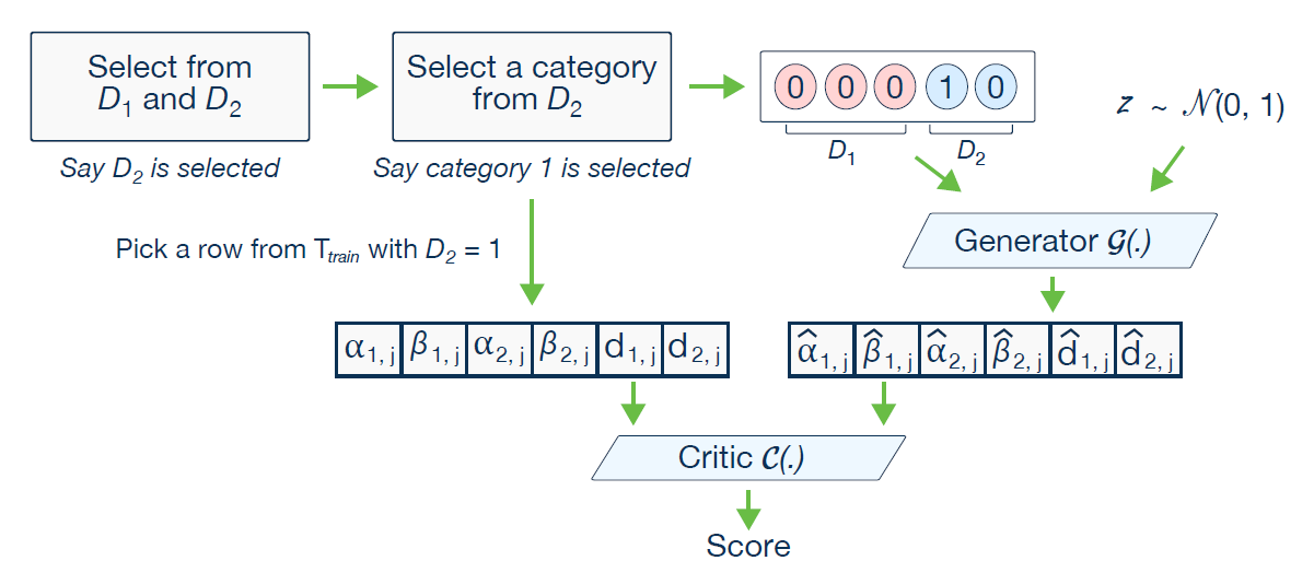
이를 달성하기 위해 저자들은 다음의 step들을 제시한다:
1)$N_d$ zero-filled mask vectors 들을 생성한다. $\mathbf{m}_i = [\mathbf{m}_i^{(k)}]_{k=1...|D_i|}$, for $i = 1,\ldots,N_d$,
- $i$번째 Discrete Column $D_i$에 대해 mask vector $\mathbf{m}_i$가 대응된다.
- mask vector $\mathbf{m}_i$의 각 원소는 해당 Column $D_i$의 category에 대응된다.
2) 총 $N_d$개의 Discrete Column 중에서 $D_i$를 random하게 선택한다.
- $i^{*}$: random하게 선택된 column index (몇 번째 column 인지)
- 아래의 그림에서 2번째 Column이 선택됐으므로, $i^* = 2$
3) random하게 선택된 $D_{i*}$ column에서 PMF를 construct한다.
- 각 value의 probability mass는 해당 column의 log(frequency) 이다.
4) $k^{*}$를 위의 PMF에서 random하게 선택된 class(category)라 하자.
- 아래의 그림에서 2번째 Column의 1번째 Class가 선택됐으므로 $k^* = 1$이다.
5) $k^{*}$ 번째 component에 해당하는 mask를 1로 설정한다. $\mathbf{m}_{i*}^{(k^*)} = 1$
6) Conditional Vector $cond$를 계산한다.
$$\text{cond} = \mathbf{m}_1 \oplus \ldots \oplus \mathbf{m}_{N_d}$$
따라서 $[00010]$으로 표현되는 conditional vector를 생성할 수 있게 된다.
위의 그림은 본 논문에서 CTGAN의 전체 과정을 나타낸 그림이다.
이렇게 training-by-sampling 을 통해 학습을 진행할 경우, discrete column에 대하여 각 category 별로 기존 데이터의 빈도와 비슷하게 학습이된다.
4.4) Network Structure
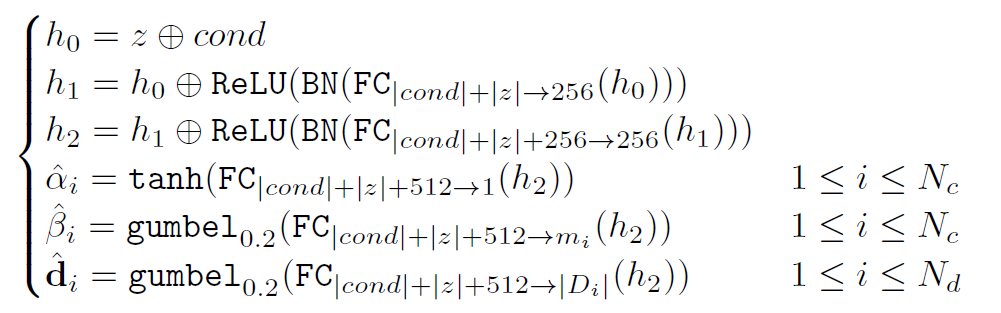
앞서 말한 내용들을 모두 정리하여 만든 generator 의 구조는 아래와 같다.
latent vector ($z \oplus cond$) 에서 시작하여 2개의 hidden layer(FC)를 거치고 난 뒤, $\alpha_i, \beta_i, \mathbf{d}_i$ 의 값을 구하게 된다.
각 FC Layer를 거친 후에 Batch Normalization과 ReLU Activation을 거쳐 Residual Network를 통과시켰다.
$\alpha$은 scalar 값이므로 activation 함수로 tanh 를 사용하였고, $\beta$와 $\mathbf{d}$는 vector 형식의 데이터이므로 다중 class 에 대한 classification이 가능한 gumbel sofmax 함수를 사용하였다.
학습에 사용된 loss는 Generator loss로, one-hot encoding된 벡터 m과 d 사이의 cross-entropy loss를 사용하게 된다.
Conditional Generator $\mathcal{G}(z, cond)$은 다음과 같은 구조를 가진다.
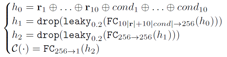
또한 discriminator (여기에서는 critic) 의 구조는 아래의 그림과 같다.
PacGAN의 구조를 사용했는데, mode collapse를 피하기 위해 하나의 pac에 10개의 sample과 conditional vector들을 넣었다. (pac size 10)
결국 마지막 레이어에서는 1개의 노드만이 남게 되며 real 데이터라면 1, fake 데이터라면 0으로 예측하게 된다. 학습에는 WGAN loss가 사용되며 optimizer로는 Adam을 이용한다.
Critic $\mathcal{C}(\mathbf{r}_1, ... , \mathbf{r}_{10}, cond_1, ... , cond_{10})$은 다음과 같은 구조를 가진다.
4.5) TVAE Model
GAN 뿐 아니라 VAE에도 해당 방식을 적용할 수 있다.
구조는 아래의 그림과 같다.
동일한 preprocessing 방식을 사용했으나, 다른 loss function을 이용했다.
cross entropy를 사용했던 Critic loss와 다르게 ELBO loss를 사용했다.
- $\alpha_{i, j}$: Gaussian Distribution을 따른다.
- $\mathbf{r}_j$: join distribution of $2N_c + N_d$
- $\beta_{i, j}, \mathbf{d}_{i, j}$: Categorical PMF를 따른다.


![[Paper Review] Image Super-Resolution via Iterative Refinement (SR3)](/content/images/size/w960/2024/09/-----2024-09-10-203649.png)
![[Paper Review] Diffusion Models Beat GANs on Image Synthesis](/content/images/size/w960/2024/07/Screenshot-2024-08-01-at-05.49.39.png)
![[Paper Review] CTAB-GAN: Effective Table Data Synthesizing](/content/images/size/w960/2024/07/Screenshot-2024-07-28-at-07.39.16.png)
![[Paper Review] Denoising Diffusion Implicit Models (DDIM)](/content/images/size/w960/2024/07/-----2024-07-24-174331.png)