[Paper Preview] Denoising Diffusion Probabilistic Models

이번 DDPM을 Review하며 참고한 자료들은 다음과 같다.

[개념 정리] Diffusion Model

GAN, VAE 와 같은 생성 모델(Generative Model) 중 하나로써, 2022년에 이슈가 되었던 text-to-image 모델인 Stable-Diffusion, DALL-E-2, Imagen의 기반이 되는 모델입니다. 많은 논문에서 Diffusion Model이 인용되지만 수식이 어려워서 간단하게 개념을 이해하고 넘어가기가 어렵습니다. 때문에 필요에 따라 깊이 별로 내용을 파악 할 수 있도록 글을 써봤습니다. Diffusion Model 이란? 입력 이미지에 (정규 분포를 가진) Noise를 여러 단계에 걸쳐 추가하고, 여러 단계에 걸쳐 (정규 분포를 가진) Noise를 제거함으로써, 입력 이미지와 유사한 확률 분포를 가진 결과 이미지를 생성하는 모델입니다. (그림 출처 : link1 , l…

TISTORYxoft

Diffusion Model 설명 - 기초부터 응용까지

Diffusion Model의 기초부터 응용까지 살펴봅니다. 기초 부분에서는 Diffusion Model의 동작 방법, Architecture, Loss Function을 살펴봅니다. 응용 부분에서는 다양한 Diffusion Model을 알아봅니다.

FFightingFfightingseok

[Paper Review] Denoising Diffusion Probabilistic Models

[발표자]고려대학교 산업경영공학과 DSBA연구실 석사과정 김정섭[발표 요약 및 Overview]- 2015년 제시된 Diffusion process 기반 비지도 학습 방법론을 기초로 함- Diffusion process의 Reverse 과정(Denoising)을 학습함으로써 주어진…

YouTube

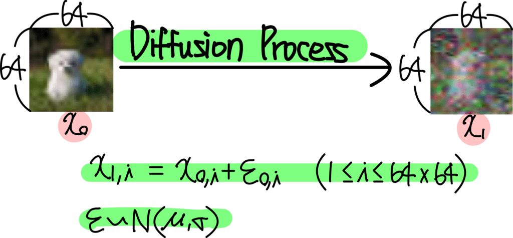
0. Diffusion Model

Forward Diffusion Process를 통해 매 time step마다 Input Image의 모든 pixel에 Gaussian Noise $\varepsilon_{\theta}$를 추가하고,

Reverse Denoising Process를 통해 매 time step마다 추가된 Gaussian Noise $\varepsilon_{\theta}$를 제거함으로써,

Input Image와 유사한 확률분포를 가지는 Result Image를 생성하는 모델이다.

Input Image에서 Gaussian Noise가 서서히 확산되기에 Diffusion(확산)이라는 이름이 붙었다고 한다.

• Forward Diffusion Process: Input Image에 fixed(고정된) Gaussian Noise가 더해진다.
• Reverse Denoising Process: Result Image에 learned(학습된) Gaussian Noise가 빼진다.

Diffusion Model의 목적은

Forward Diffusion Process를 거친 Result Image의 확률분포를 Reverse Denoising Process를 통해 Input(Real) Image의 확률분포와 유사하게 만드는 것이다.

이를 달성하기 위해 Reverse Denoising Process에서 학습을 통해 Noise 생성 확률 분포 Parameter인 Mean $\mu$, Standard Deviation $\sigma$를 조절한다.

1. Diffusion Preview

"Diffusion"이라 함은 "확산" 현상을 의미한다.

아래의 그림을 보면 지정된 space안의 공기 분자들이 시간이 지남에 따라 Diffusion Process를 통해 전체 space안에 고르게 분포하는 것을 알 수 있다.

이때, 공기 분자 하나의 움직임을 관찰해보자.

매우 짧은 time step (sequence)동안 하나의 분자가 움직이는 Movement는 Gaussian Distribution을 따른다.

위의 그림은 매우 짧은 time step $t$ 단위로 분자 하나의 Movement $m_{t}$ 를 표시한 것이다. 이때, Movement $m_{t}$는 Gaussian Distribution을 따르므로 $m_{t} \sim N(\mu, \sigma)$으로 표현가능하다.

즉, 매시간 $t$마다 각 분자들은 Gaussian Distribution에 의한 Movement를 수행하는데 만약 이 Movement들을 예측해낼 수 있다면 Reverse Diffusion Process에 의해 Noisy 하지 않은 원상태를 구현할 수 있다.

이제, 위의 Diffusion Process를 Image에 적용해보자.

매 time step $t$마다 Molcule(분자)에 Gaussian Distribution을 따르는 Noise Movement $m_{t}$ 가 더해져 최종 Movement가 결정된다. 반면에 Image에서는 각 pixel에 Gaussian Noise $\varepsilon_{\theta}$ 가 더해져 그 다음 time step의 pixel이 된다.

위의 내용들을 종합하여 수식으로 나타내면 다음과 같다:

• $x_{0}$: 원본 image ($N \times N$ size)
• $x_{1}$: 다음 time step의 image
• $i$: image에 위치한 pixel의 position (index)

이미지의 각 pixel position에 대해 다음과 같이 식이 작성된다.

$x_{1, i}$ = $x_{0, i} + \varepsilon_{o, i}$ ($1 \leq i \leq N^{2}$)

$\varepsilon \sim N(\mu, \sigma)$

위의 예시는 $64 \times 64$의 image의 모든 pixel value에 Gaussian Noise $\varepsilon_{\theta}(x_{t}, t)$을 추가해주는 과정이다.

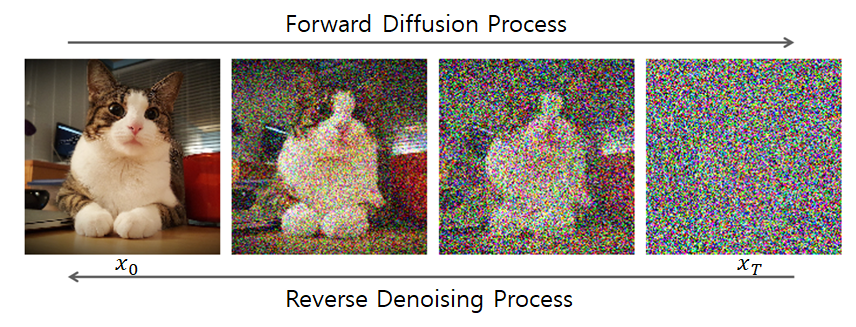
이러한 과정을 수많은 time step $t$ 마다 반복하여 완전한 Noise Image로 만들어준다. 이는 아래의 그림을 통해 설명가능하다.

위 과정은 Diffusion Forward Process라 한다. 매 time step $t$ 마다 이전 이미지 $x_{t-1}$의 모든 pixel에 fixed Gaussian Noise $\varepsilon$를 추가하여 time step $t$ 에서의 이미지 $x_{t}$를 형성한다.

위의 과정을 반복하여 최종 time step $T$에서는 $x_{T}$가 완전한 Noise Image가 되어있음을 알 수 있다.

이때, 매 time step $t$에서 첨가된 Gaussian Noise $\varepsilon_{\theta}(x_{t}, t)$을 계산할 수 있다면 Noise Image $x_{T}$에서 Real Image (Data) $x_{0}$로 Noise를 제거하면서(Subtraction) 되돌리는 것이 가능하다.

이는 Image Generation이 가능하다는 말을 뜻한다.

• Input: $x_{T}$ (random noise image)
• Output: $x_{0}$ (real / desired image)
• Process: Reverse Diffusion Process

정리해보면, Diffusion Model은 time step $t$에서의 image $x_{t}$를 입력으로 받아, 각 pixel별로 추가된 Gaussian Noise $\varepsilon_{\theta}(x_{t}, t)$를 예측하는 것이다.

해당 Noise $\varepsilon$를 subtract하면 이전 time step $t-1$에서의 image (less noisy image)로 변환가능하기에, $x_{T}$에서 위의 과정을 반복해 나가면 결국 real image (Data) $x_{0}$를 구현해낼 수 있다.

Diffusion Model이 갖춰야 하는 4가지 Condition들은 다음과 같다:

1. Input: Image or Noisy Image (3D Tensor 형태 or 2D Array 형태여야 한다)
2. Time step: 몇 번째 Process인지를 의미하는 $t$도 주어져야 한다.
3. Condition: 추가 Condition이 있다면 이 조건 또한 Diffusion Model에 주어져야 한다.
   1. Condition이란 특정 class 정보, 또는 생성한 이미지를 표현할 Text 정보 등등이 해당한다.
   2. Classifier Guidance를 통해 주어질 수도 있고, 바로 Diffusion Model에 주어질 수도 있다.
4. Output: Input과 동일한 Shape여야 한다.
   1. value는 각 pixel별로 첨가된 Noise값을 의미한다.
   2. Diffusion Model에 따라 Noise값 자체를 예측할지, Noise의 $\mu, \sigma$등을 예측할지는 조금씩 다르지만, Noise를 예측한다고 이해하면 큰 문제는 없다.

위 그림은 일반적인 Diffusion Model의 Architecture를 표현한 그림인데, Diffusion Model은 U-Net 구조를 띄고 있는 것을 알 수 있다.

• U-Net의 Structure 특성상 이는 Input과 동일한 Resoution을 가지는 Output을 내기에 용이하다.
• time step $t$ 를 별도로 입력받는다.
• 위의 구조는 대부분의 Diffusion Model에서 공통적으로 사용되고 있는 구조다.

앞서 말했듯, Diffusion Model은 time step $t$에서

• Input: Noisy Image $x_{t}$
• Output: Gaussian Noise $\varepsilon_{\theta}(x_{t}, t)$

위와 같음을 알 수 있다.

따라서, 각 pixel마다 첨가된 Gaussian Noise $\varepsilon_{\theta}$을 예측하는데, Loss Function은 아래와 같이 표현가능하다.

• $\varepsilon$: Ground Truth (Real Noise)
• $\varepsilon_{\theta}$: Diffusion Model이 예측한 Noise

위의 두 항이 같아지도록 Diffusion Model을 학습시킨다.

2. Diffusion Introduction & Prerequisite

최근 Diffusion Model을 여러 분야에 활용하려는 노력이 일고 있다.

이상탐지 방법론의 Backbone Model로 사용되거나 GAN, VAE와 결합하기도 한다.

특히나 Text-to-Image Generation 분야에 많이 활용되고 있다.

뿐만 아니라 Image, Audio 등 다양한 분야의 데이터셋에 대해서도 높은 퀄리티의 Generation을 수행한다.

1) What is Diffusion?

Diffusion 이라는 개념은 Thermodynamics(물리 통계 동역학)에서 시작했는데, 특정 물질이 시간이 지남에 따라 "확산"되면서 같은 농도로 바뀌는 현상을 의미한다.

이는 물질들의 분포가 서서히 와해되는 과정으로도 볼 수 있으며, 2015년도의 ICML에서 발표된 Deep Unsupervised Learning using Nonequilibrium Thermodynamics가 Diffusion 논문의 시초라고이다.

위의 그림은 Forward Diffusion Process를 Alphabet 'e'에 적용하여 시간이 지남에 따라 각 sample data의 point들을 Gaussian Noise로 변키는 과정을 보여준다.

이때, $t$는 discrete한 step을 지칭한다.

Diffusion Model을 이해하기 위해서는 Markov Chain에 대한 개념이 선행되어야 한다.

2) Prerequisite

Markov Chain은 Markov 성질을 갖는 Dicrete한 확률과정이라 할 수 있다.

Discrete한 확률과정: Discrete Time $t=0, 1, 2, ...$ 속에서의 확률적 현상

여기서 Markov 성질이라 함은 "특정 상태($t+1$)의 확률은 오직 현재($t$)의 상태에만 의존한다." 으로 볼 수 있다.

$$q(\mathbf{x}_T|\mathbf{x}_{T-1}) = q(\mathbf{x}_T|\mathbf{x}_{T-1}, \mathbf{x}_{T-2}, ..., \mathbf{x}_1, \mathbf{x}_0)$$

Normalizing Flow는 Neural Network 기반 확률적 생성 모델 중 하나이다.

Flow Model은 Latent Variable 기반 확률적 생성모형으로서, latent variable($z$) 획득에 변수변환 공식을 사용한다.

$$p_x(x) = p_z(z)|\frac{dz}{dx}|$$

Input data sample $x$를 Prior Gaussian 과 같은 well-known Distribution으로 mapping하는 함수 $f$를 학습한다.

이는 한 번에 이루어지지 않고, 단계별로 작은 변화들을 step-by-step으로 학습하도록 한다.

이렇게 학습한 function $f$의 inverse function $f^{-1}$ Prior Distribution을 우리가 원하는 Input Data의 Distribution으로 예측하는 Model을 설계한다.

3) Probabilistic Generative Models

Diffusion Model은 iterative transformation을 활용한다는 점에서 Flow-based model과 유사하다.

또한, Variational Lower Bound(ELBO) Concept을 이용한다는 점에서 VAE와 유사하기도 하다.

최근에는 Diffusion Model에 Adversarial training을 활용하는 연구도 진행되고 있다. Diffusion-GAN, 2022

대부분의 Probabilistic Generative Model의 경우에는 well-known(tractable) Distribution (Gaussian, Uniform 등)에서 확보한 latent variable $z$으로 Generative Process를 시작한다.

Simple Distribution을 Input으로 받아 Trained Model을 통해 우리가 원하는 Data의 Complex Distribution으로 변환하는 것을 목표로 한다.

따라서, Probabilistic Generative Model에서 필요로 하는 것은 아래 2개 이다.

• Input: Latent Variable $z$
• Model: Simple, Tractable distribution을 우리가 원하는 Data의 Complex distribution으로 mapping할 수 있는 Model

VAE는 Decoder를 이용해 latent variable을 구하고자 하는 특정 distribution으로 mapping한다.

Encoder Network를 Model Architecture에 추가함으로써, Latent variable $p_{\theta}(z)$ / Encoder $q_{\phi}(z|x) \approx p_{\theta}(z|x)$/ Decoder $p_{\theta}(x|z)$를 모두 학습하며 Marginal Likelihood $p_{\theta}(x)$를 구하고자 한다.

$$p_{\theta}(x) = \frac{p_{\theta}(z)p_{\theta}(x|z)} {q_{\phi}(z|x)}$$

GAN은 Generator가 매우 simple한 latent variable을 구하고자 하는 data의 distribution으로 mapping하고자 한다.

Generator가 원하는 data의 distribution으로 mapping하기 위해 Discriminator를 도입하여 adversarial learning을 통해 2개의 Network를 training한다.

Flow-based Model도 마찬가지로 simple, tractable한 distribution을 구하고자 하는 data의 complex distribution으로 mapping하고자 한다.

이러한 과정에서 기존의 data에서 well-known distribution으로 mapping하는 함수 $f$를 학습하고 chain으로 엮어 chain of functions (forward flow) 를 설계한다.

생성시에는 그 역함수인 $f^{-1}$를 이용하여 chain of functions (inverse flow) 을 통해 Generative Model을 설계한다.

Diffusion Model도 마찬가지로 Prior Distribution을 $P(z)$ 우리가 원하는 Marginal Distribution $P(x)$으로 Mapping하도록 학습한다.

DDPM에서 구상하는 전략은 Forward Diffusion Process에서는 Training을 하지 않는다. 즉, Fixed Noise를 매 time step마다 추가해주고 있다고 생각하면 된다.

다시 말해, DDPM에서 실제 Training되는 process는 오직 Sampling Process(Reverse Denoising Process)로 한정된다.

그리고 이때, Reverse Desnoising Process에서 사용되는 $p_{\theta}(x|z)$를 학습하기 위해 Forward Diffusion Process의 $q(z|x)$를 활용한다.

Forward / Reverse Process 모두 markov chain을 이용하여 distribution을 구상한다.

3. Diffusion Model

1) Diffusion Model Overview

Diffusion Model은 Input Data에 fixed noise를 추가하는 Forward Diffusion Process를 통해 Gaussian Noise를 만든 후,

Reverse Denoising Process를 통해 Gaussian Noise에서 Input Data의 distribution과 유사한 확률분포를 mapping하기 위해 subtract하는 Noise를 학습한다.

이때, Forward Diffusion Process는 fixed gaussian noise를 주입하기 때문에 $q(\mathbf{x}_{t}|\mathbf{x}_{t-1})$의 distribution은 알아서 결정된다.

다만, Reverse Denoising Process에서 사용되는 $q(\mathbf{x}_{t-1}|\mathbf{x}_{t})$는 Inference(generation)과정에서 사용이 불가능하다.

즉, $q(\mathbf{x}_{t}|\mathbf{x}_{t-1})$를 안다고 해서 direct하게 $q(\mathbf{x}_{t-1}|\mathbf{x}_{t})$으로의 변환이 불가능하다는 뜻이다.

따라서 Reverse Denoising process가 training을 통해 구현되어야 한다는 idea가 나온 것이다.

여기서 Forward/Reverse process모두 Gaussian Distribution을 따른다는 점이 반영된다.

여기서 $q(\mathbf{x}_{t-1}|\mathbf{x}_{t})$는 intractable하기에, $p_{\theta}(\mathbf{x}_{t-1}|\mathbf{x}_{t}) \approx q(\mathbf{x}_{t-1}|\mathbf{x}_{t})$를 만족하는 tractable한 $p_{\theta}(\mathbf{x}_{t-1}|\mathbf{x}_{t})$를 도입한다.

결국 Reverse Denoising Process를 통해 $p_{\theta}(\mathbf{x}_{t-1}|\mathbf{x}_{t}) \approx q(\mathbf{x}_{t-1}|\mathbf{x}_{t})$가 되도록 학습시킨다면,

subtract하는 gaussian noise를 예측할 수 있어 기존의 input data의 distribution과 유사한 distribution을 갖는 data를 생성할 수 있게 된다.

다만 이러한 transformation을 하나의 단일 step으로 표현하는 것은 매우 어려운 문제이다.

그렇기에 위의 step을 작은 step들로 잘게 나누어 학습한다.

따라서 Markov chain을 이용하여 discrete time step에서의 distribution을 곱함으로써, initial $\mathbf{x}_{0}$, 특정 $\mathbf{x}_{t}$ time step 간의 conditional distribution $q(\textbf{x}_{1:T} | \textbf{x}_{0}), p_{\theta}(\mathbf{x}_{0:T})$을 구할 수 있게 된다.

DDPM에서는 위의 step을 1000번으로 나누어 학습하며, 해당 과정인 $p_{\theta}(\mathbf{x}_{t-1}|\mathbf{x}_{t})$의 학습은 결국 estimating large number of small perturbations으로 볼 수 있다.

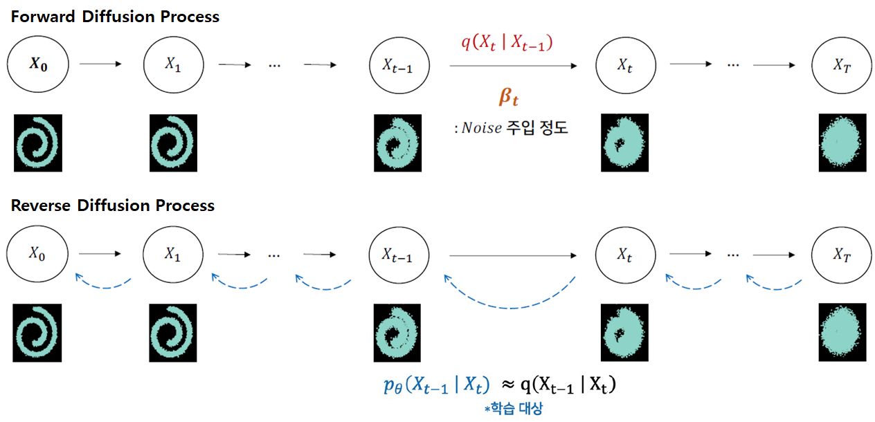
2) Forward Diffusion Process

이 Forward Process는 $q(\mathbf{x}_{t}|\mathbf{x}_{t-1})$의 Markov Chain으로 구성되어 있다.

다만, Forward Diffusion Process에서는 Diffusion Model이 학습되지 않는다.

단지 사전에 정의된 Fixed Gaussian Noise를 noise injection parameter $\beta_{t}$에 맞춰 주입할 뿐이다.

Noise Injection Parameter $\beta_{t}$는 아래의 수식을 통해 forward process에 반영된다.

$q(\textbf{x}_{t}|\textbf{x}_{t-1}) = N(\textbf{x}_{t}; \sqrt{1-\beta_{t}} \textbf{x}_{t-1}, \beta_{t}\textbf{I})$

Noise Injection Parameter $\beta_{t}$는 time step이 지남에 따라 점진적으로 커지도록 설계된다.

$\beta_{t}$의 설계 방법은 크게 3가지가 있다.

• Linear Schedule
• Quad Schedule
• Sigmoid Schedule

def make_beta_schedule(schedule="linear", n_timesteps=1000, start=1e-4, end=0.02):
    if schedule == "linear":
        return torch.linspace(start, end, n_timesteps)
    elif schedule == "quad":
        return torch.linspace(start**0.5, end**0.5, n_timesteps) ** 2
    elif schedule == "sigmoid":
        return torch.sigmoid(torch.linspace(-6, 6, n_timesteps)) * (end - start) + start

위와 같이 beta scheduler를 구현할 수 있다.

quadratic scheduling이나 sigmoid scheduling은 $x^2$ or sigmoid function의 $y$값에서 start ~ end까지 n_timesteps만큼 나눈거라 생각하면 된다.

위의 3개의 scheduling case에 대해 각각 아래와 같이 결과가 나온다.

다만 현재는 cosine scheduling을 가장 많이 사용하고, 성능이 좋은 추세이다.

3개의 Dataset(Swiss-roll, MNIST, CELEB A)에 대해 각각 Gaussian Noise가 주입되며 최종적으로는 Noisy한 Image가 되는 것을 볼 수 있다.

$$q(\textbf{x}_{t}|\textbf{x}_{t-1}) = N(\mathbf{x}_t ; \mu_{\mathbf{x}_t}, \Sigma_{\mathbf{x}_t} ) = N(\textbf{x}_{t}; \sqrt{1-\beta_{t}} \textbf{x}_{t-1}, \beta_{t}\textbf{I})$$

이 식을 Noise Injection parameter인 $\beta_{t}$(fixed)를 포함하여 다르게 표현하면, 이전 상태($\mathbf{x}_{t-1}$)의 이미지가 $\beta_{t}$만큼 다른 pixel을 선택하게 하고, $\sqrt{1-\beta_{t}}$ 만큼 이전 pixel값을 선택하게 하는 식으로 정의 할 수 있다.

$t$가 점점 증가함에 따라 $\beta_{t}$가 커짐으로써 Noise가 강해진다.

Forward과정에서 $\beta_{t}$는 각 time step에서 Injection되는 Noise가 고정(fixed)되어 있지만, 확률 분포를 따르기 때문에 마지막 상태($\mathbf{x}_{T}$)의 결과가 항상 다를 수 있다.

• $q(\mathbf{x}_{t}|\mathbf{x}_{t-1})$: 이전 상태($x_{t-1}$) 주어졌을 때 현재 상태($x_{t}$)가 될 확률분포 Tractable
• $q(\mathbf{x}_{t-1}|\mathbf{x}_{t})$: 현재 상태($x_{t}$) 주어졌을 때 이전 상태($x_{t-1}$)가 될 확률분포 Intractable

그리고 이를 Reparameterization Trick을 이용하여 Sampling한 $\mathbf{x}_t$에 대해 식을 작성해보면 다음과 같다.

$$\mathbf{x}_t = \sqrt{1-\beta_t}\mathbf{x}_{t-1} + \sqrt{\beta_t}\boldsymbol{\epsilon}, \quad \boldsymbol{\epsilon} \sim \mathcal{N}(0, \mathbf{I})$$

- $\text{Var}(\varepsilon) = \mathbf{I}$

- $\mathbf{x}_{t}$는 Gaussian Distribution에서 sampling했기 때문에 Covariance Matrix의 각 element인 $\beta_{t}$에 $\varepsilon$를 곱하면 된다.

- Identity Matrix $I$를 $\varepsilon$에 곱하는 것이 아니라 $\mathbf{x}_{t}$를 sampling했기에 standard deviation value $\sqrt{\beta_{t}}$를 가지고 $\varepsilon$에 바로 곱해주면 된다.

이러한 Forward Process를 코드로 구현하면 다음과 같다:

def forward_process(x_start, n_steps, noise=None):
    """_summary_

    Diffuse the data (t==0 means diffused for 1 step)

    x_start: tensor = data set at start step(X_0)
    n_steps: int = number of convert iterations in the diffusion process
    noise: tensor = noise tensor to be added to the data set (scheduled)
    """
    x_sequence = [x_start]  # inital 'x_sequence' is the data set at the start step
    for n in range(n_steps):
        beta_t = noise[n]
        x_prev = x_sequence[-1]
        epsilon_prev = torch.randn_like(x_prev)
        x_next = torch.sqrt(1 - beta_t) * x_prev + torch.sqrt(beta_t) * epsilon_prev
        x_sequence.append(x_next)

    return x_sequence

사실 Diffusion Model은 latent variable $z$를 많이 가져가는 Model인데, $\mathbf{x}_{0}$을 제외한 $\mathbf{x}_{1}, \mathbf{x}_{2}, ..., \mathbf{x}_{T}$들을 latent variable로 간주한다.

conditional gaussian distribution에서 sampling한 latent variable $q(\mathbf{x}_{t}|\mathbf{x}_{t-1})$으로 볼 수 있다.

Noise 주입의 정도의 차이가 있지만, 모두 Noise가 주입된 latent variable로 볼 수 있다.


이렇게 다수의 latent variable들 $\mathbf{x}_{1}, \mathbf{x}_{2}, ..., \mathbf{x}_{T}$을 간주한다는 점에서 Hierarchical VAE와 유사하다.

이렇게 본다면, Forward Diffusion Process는 결국 $\mathbf{x}_0$을 조건부로 Latent Variables $\textbf{x}_{1:T}$를 생성해내는 과정이라 볼 수 있다.

Forward Diffusion Process

$$q(\textbf{x}_{1:T} | \textbf{x}_{0}) = \prod_{t=1}^{T} q(\textbf{x}_{t}|\textbf{x}_{t-1})$$

그리고 마지막 time step $\mathbf{x}_{T}$에서의 latent variable은 매우 많은 Gaussian Noise가 주입된 상태이므로 pure isotropic gaussian 으로 볼 수 있다.

결국에는 Foward Diffusion Process는 Conditional Distribution들의 Markov Chain 을 통해 다수의 latent variable들을 얻어가는 과정이다.

3) Reverse Denoising Process

Reverse Desnoising Process는 기존 주입한 Gaussian Noise로 인해 만들어진 Noisy Image에서

각 time step별 inject된 Noise를 예측하여 subtract해줌으로써 기존의 original image의 distribution과 유사한 distribution을 예측하도록 noise를 학습한다.

Physical Intuition에 의해, Reverse Step 또한 마찬가지로 각 Probability Distribution $q(\mathbf{x}_{t-1}|\mathbf{x}_{t})$이 Intractable한 Gaussian Process라고 볼 수 있다.

다만, forward process에서는 $q(\mathbf{x}_{t}|\mathbf{x}_{t-1})$가 tractable distribution이었으나 reverse process에서는 $q(\mathbf{x}_{t}|\mathbf{x}_{t-1})$가 intractable하다.

따라서 intractable한 $q(\mathbf{x}_{t}|\mathbf{x}_{t-1})$를 tractable한 Gaussian Distribution인 $p_{\theta}(\mathbf{x}_{t-1}|\mathbf{x}_{t})$을 통해 근사시켜야 하는데,

이를 parameter $\mu_{\theta}(\mathbf{x}_t, t), \Sigma_{\theta}(\mathbf{x}_{t}, t))$ 들을 training을 통해 구한다.

Gaussian Noise로부터 시작을 해서,

$$p(\mathbf{x}_T) = \mathcal{N}(\mathbf{x}_T; 0, \mathbf{I})$$

확률분포 $q$가 주어졌을 때, 이 확률 분포를 가장 잘 모델링하는 확률 분포 $p_{θ}$를 찾는다.

$$p_{\theta}(\mathbf{x}_{t-1}|\mathbf{x}_{t}) = \mathcal{N}(\mathbf{x}_{t-1}; \mu_{\theta}(\mathbf{x}_t, t), \Sigma_{\theta}(\mathbf{x}_{t}, t))$$

가 되는데, 이때

• $ \mu_{\theta}(\mathbf{x}_t, t)$: Mean
• $\Sigma_{\theta}(\mathbf{x}_{t}, t)$: Variance

두 개의 파라미터를 어떻게 Train시킬지가 굉장히 중요해진다.

Reverse Denoising Process

$$p_{\theta}(\mathbf{x}_{0:T}) = p(\mathbf{x}_{T})\prod_{t=1}^{T} p_{\theta}(\mathbf{x}_{t-1}|\mathbf{x}_{t})$$

위와 같이 probability distribution들의 joint의 형태로 표현이 가능하다.

• $q(\textbf{x}_{1:T} | \textbf{x}_{0}) = \prod_{t=1}^{T} q(\textbf{x}_{t}|\textbf{x}_{t-1})$: Forward Diffusion Process
• $p_{\theta}(\mathbf{x}_{0:T}) = p(\mathbf{x}_{T})\prod_{t=1}^{T} p_{\theta}(\mathbf{x}_{t-1}|\mathbf{x}_{t})$: Reverse Denoising Process

각 time step $t$에서의 reverse process에 의해 추출된 gaussian noise의 $\mu, \sigma$는 다음과 같이 코드로 작성할 수 있다.

def p_mean_variance(model, x, t, device):

    # make model prediction
    out = model(x, t.to(device))

    # extract the mean and variance
    mean, log_var = torch.split(out, 2, dim=-1)
    var = torch.exp(log_var)
    return mean, log_var

위와 같은 학습이 다 완료되었다고 했을 때, Reverse Denoising Process는 아래의 GIF를 통해 원래 이미지와 비슷한 형태로 복원되는 것을 확인할 수 있다.

위의 Reverse process에서 Diffusion Model을 학습할 때 사용되는 Loss에 대해 살펴보자.

최종 DDPM Loss는 다음과 같이 작성할 수 있다.

$$L = \mathbb{E}_q\left[D_\text{KL}(q(x_T|x_0)||p(x_T)) + \sum_{t>1} D_\text{KL}(q(x_{t-1}|x_t, x_0)||p_\theta(x_{t-1}|x_t)) - \log p_\theta(x_0|x_1)\right]$$

결국 이는 Density Estimation의 관점에서 아래의Negative Log likelihood를 Minimize하자는 의도에서 시작한다.

$$\mathbb{E}_{x_T \sim q(x_T|x_0)}[-\log p_\theta(x_0)]$$

여기서 VAE와 Diffusion Model의 구조를 비교해보자.

VAE는 기본적으로 하나의 latent variable $z$을 추출해내지만, Diffusion Model의 경우 각 time step $t$에 따른 state에 의해 multiple latent variable $\mathbf{x}_{t}$을 추출한다.

둘은 latent variable의 수에 따른 차이가 존재하고, 이는 Loss를 구성하는 term에 영향을 미친다.


또한, Diffusion Model은 latent variable의 size가 input data의 size와 동일하다.

VAE와 Diffusion Model 모두 Loss Term에 Reconstruction, Regularization Term을 갖게 된다.

VAE Loss

$$Loss_{VAE} = D_{KL}(q(z|x)||p_\theta(z)) - E_{z\sim q(z|x)}[\log P_\theta(x|z)]$$


- Regularization: $D_{KL}(q_{\phi}(z|x)||p_\theta(z))$


- Reconstruction: $E_{z\sim q(z|x)}[\log P_\theta(x|z)]$

Diffusion Loss


$$Loss_{Diffusion} = D_{KL}(q(z|x_0)||P_\theta(x_0|z)) - E_{z\sim q(z|x)}[\log P_\theta(z)]$$


$$= D_{KL}(q(z|x_0)||P_\theta(z)) + \sum_{t=2}^T D_{KL}(q(x_{t-1}|x_t,x_0)||p_\theta(x_{t-1}|x_t)) - E_q[\log P_\theta(x_0|x_1)]$$


- Regularization: $D_{KL}(q(z|x_0)||P_\theta(z))$ Forward Process


- Reconstruction: $E_q[\log P_\theta(x_0|x_1)]$ Reverse Process


- Denoising Process:$ \sum_{t=2}^T D_{KL}(q(x_{t-1}|x_t,x_0)||p_\theta(x_{t-1}|x_t))$ Reverse Process

결국 차이를 보이는 부분은 Denoising Process 부분이다.

Reverse Denoising Process 부분을 학습하도록 guide하는 loss term이 녹색 box 부분이다.

$ \sum_{t=2}^T D_{KL}(q(x_{t-1}|x_t,x_0)||p_\theta(x_{t-1}|x_t))$ Term은 tractable하면서도 잘 학습될 수 있다.

$$q(x_{t-1}|x_t, x_0) = q(x_t|x_{t-1}, x_0)\frac{q(x_{t-1}|x_0)}{q(x_t|x_0)}$$


에서 $q(x_{t-1}|x_t, x_0)$을 구성하는 3개의 항이 모두 tractable하다.

결국에는 $q(\mathbf{x}_{t-1}|\mathbf{x}_t,\mathbf{x}_0)$를 $p_\theta(\mathbf{x}_{t-1}|\mathbf{x}_t)$를 통해 approximation 할 수 있다.

따라서 전체 Diffusion Process를 위와 같이 표시한다면, 3개의 term이 각각 어떤 부분을 담당하고 있는지 확인해볼 수 있다.

기존의 $p_\theta(\mathbf{x}_{t-1}|\mathbf{x}_t)$는 $q(\mathbf{x}_{t-1}|\mathbf{x}_t)$가 intractable하기 때문에 도입하여 approximation하려는 것이 아니였나?


그런데 왜 approximation의 대상이 intractable한 $q(\mathbf{x}_{t-1}|\mathbf{x}_t)$가 아니라 tractable한 $q(\mathbf{x}_{t-1}|\mathbf{x}_t,\mathbf{x}_0)$으로 바뀌었지?


물론 Loss Function에서 도출된 것은 알고 있으나, approximation을 수행하는 목적이 달라지면 안 되는거 아닌가?


tractable한 항으로 approximate하는게, 궁극적으로 intractable한 항으로 approximate하는 걸 달성할 수 있도록 어떻게 연결되는 거지?

Loss Term을 좀 뜯어보면 다음과 같은 결론을 내릴 수 있다:

위 식 전개의 6)에서 주어진 Loss를 Minimize시키기 위해서는 $D_{\text{KL}}(q(\mathbf{x}_{t-1}|\mathbf{x}_t) \parallel p_\theta(\mathbf{x}_{t-1}|\mathbf{x}_t))$도 Minimize시켜야 한다.

즉, 이미 training되는 $p_\theta(\mathbf{x}_{t-1}|\mathbf{x}_t)$ distribution을 intractable한 $q(\mathbf{x}_{t-1}|\mathbf{x}_t)$ distribution으로 가까워지도록 학습하는 것이 6)에 명시되어 있다.

이제 위의 식을 6)에서 계산할 수 있는 항만 남기도록 전개해보니, 최종적으로 Denoising Matching term에서 KLD가 나와 tractable한 $q(\mathbf{x}_{t-1}|\mathbf{x}_t,\mathbf{x}_0)$으로 가까워지도록 만드는 것이다.

직접적으로는: $q(\mathbf{x}_{t-1}|\mathbf{x}_t,\mathbf{x}_0) \approx p_\theta(\mathbf{x}_{t-1}|\mathbf{x}_t)$으로 근사시킨다.

그런데 이렇게 KL Divergence를 통해 근사시키면 결국 간접적으로도 $q(\mathbf{x}_{t-1}|\mathbf{x}_t) \approx p_\theta(\mathbf{x}_{t-1}|\mathbf{x}_t)$와 같이 초기의 목적을 달성하게 된다.

결국 근본적으로 달성하는 목적은 동일하기에 tractable한 $q(\mathbf{x}_{t-1}|\mathbf{x}_t,\mathbf{x}_0)$항을 이용하여 계산을 더 용이하게 만드는 것이다.

4. DDPM Paper Review

결국 DDPM 논문에서의 설명 Flow는 다음과 같다:

1) DDPM Loss 식을 간결화한다.

• VAE ELBO에서 Loss식 유도
• Regularization Term을 제거
• Denoising Matching Term 남김

2) Learnable Parameter $\mu_{\theta}(\mathbf{x}_t, t), \Sigma_{\theta}(\mathbf{x}_{t}, t))$ 중 $\mu_{\theta}(\mathbf{x}_t, t)$만 남긴다.

• $\Sigma_{\theta}(\mathbf{x}_{t}, t))$: Time-dependent Constant
• $\beta_t, \alpha_t$로 $\Sigma_{\theta}(\mathbf{x}_{t}, t))$ 표현가능

$$\sigma_{t}^{2} \cdot I = \tilde{\beta_{t}} \cdot I$$

3) Denoising Matching Term의 KL Divergence 두 분포가 Gaussian Distribution을 따른다.

• KLD의 두 distribution이 모두 gaussian 일 때 사용하는 공식
• constant를 제거하면 결국 두 $\mu$의 차에 의한 loss가 반환

$$\mathbb{E}_q\left[\frac{1}{2\sigma_t^2} ||\tilde{\mu_t}(x_t, x_0) - \mu_\theta(x_t, t)||^2\right]$$

4) $\mu_{\theta}(\mathbf{x}_t, t)$를 reparameterization trick을 이용하여 $\epsilon$에 대한 식으로 정리한다.

• 실제 각 time step $t$에서 정해져 있지 않은 항은 Gaussian Noise $\epsilon$뿐이다.
• 그렇기에 $\mu$에 대한 식을 $\epsilon$에 대한 식으로 재정리

$$\mathbb{E}_{x_0,\epsilon}\left[\frac{\beta_t^2}{2\sigma_t^2\alpha_t(1-\alpha_t)}\left|\epsilon - \epsilon_\theta\left(\sqrt{\alpha_t}x_0 + \sqrt{1-\alpha_t}\epsilon,t\right)\right|^2\right]$$

5) $\epsilon$에 대한 loss function을 정의하고, 상수 계수를 1로 처리한다.

• time step $t$가 증가함에 따라 계수가 점차 감소
• $t$가 큰 noisy image에 가까운 시점에서는 학습의 중요도가 앞의 작은 $t$에 비해 작음
• 따라서 계수를 상수로 만들어 상대적으로 $t$가 큰 시점에서의 학습의 중요도를 올림

$$L_\text{simple}(\theta) := \mathbb{E}_{t,x_0,\epsilon}\left[\left|\epsilon - \epsilon_\theta\left(\sqrt{\alpha_t}x_0 + \sqrt{1-\alpha_t}\epsilon,t\right)\right|^2\right]$$

DDPM에서는 아래와 같이 Loss Term을 간소화 시켜 정의한다.

그렇다면 어째서 DDPM의 Loss Term이 다음과 같이 나오는지 살펴보자.

Regularization Term은 final time step $t=T$에서 latent variable이 prior gaussian $P_{\theta}(z)$를 따르도록 강제하는 역할을 한다.

다만 실제 연구를 해보니, 굳이 KL Divergence로 강제하지 않아도 매우 많은 time step $t$동안 gaussian noise를 주입하면

final time step $t=T$에서 isotropic guassian과 어느정도 유사하게 나오기에 Regularization Term을 제외해도 된다고 보았다.

위와 같이 Linear Scheduling으로 $\beta_t$를 설정하게 될 경우 최종적인 Latent variable이 충분한 isotropic gaussian을 따르는 것을 볼 수 있다.

Reverse Denoising Process에서는 각 time step $t$에서 subtract되는 gaussian noise의 $\mu, \Sigma$를 학습을 통해 예측할 필요가 있다.

먼저, 학습대상을 $\mu, \Sigma$ 중 $\Sigma$를 제외해서 가져가게 된다.

왜냐하면, 기존에 알고 있는 정보인 Noise Injection Parameter $\beta_t$를 이용하여 $\Sigma$에 대한 식으로 표현이 가능하기에 time dependent한 Constant로 처리 가능하기 때문이다.

굳이 training 해야 하는 learnable parameter로 설정할 필요가 없다.

따라서 $\sigma_{t}^{2} \cdot I = \tilde{\beta_{t}} \cdot I$으로 $t$ 시점까지 누적된 noise로 표현가능하다.

따라서 DDPM에서는 학습 대상이 $\mu_{\theta}(\mathbf{x}_t, t), \Sigma_{\theta}(\mathbf{x}_{t}, t))$ 2개에서 $\mu_{\theta}(\mathbf{x}_t, t)$ 1개로 줄어들었다.

이후 기존의 Denoising Process Loss Term $ \sum_{t=2}^T D_{KL}(q(x_{t-1}|x_t,x_0)||p_\theta(x_{t-1}|x_t))$을 $\mu_{\theta}(\mathbf{x}_t, t)$의 추정에 집중하여 다시 작성해볼 수 있다.

$$\mathbb{E}_q\left[\frac{1}{2\sigma_t^2} ||\tilde{\mu_t}(x_t, x_0) - \mu_\theta(x_t, t)||^2\right]$$

이는 Mean Function간의 차이로 귀결된다.

그리고, Denoising 과정을 이용해 위의 mean function을 변형시키고자 하는데, 이를 Denoising matching이라 한다.

Reparameterize-Trick과 Markov Chain을 이용한 sampling 식을 기존의 mean function식에 대입하여 정리하면 아래와 같이 정리할 수 있다.

$$\mathbb{E}_{x_0,\epsilon}\left[\frac{1}{2\sigma_t^2}\left|\frac{1}{\sqrt{\alpha_t}}\left(x_t(x_0, \epsilon) - \frac{\beta_t}{\sqrt{1-\bar{\alpha_t}}}\epsilon\right) - \mu_\theta(x_t(x_0, \epsilon), t)\right|^2\right]$$

결국 위의 mean function $\mu_\theta(x_t(x_0, \epsilon), t)$이 예측해야 하는 부분은 $\frac{1}{\sqrt{\alpha_t}}\left(x_t(x_0, \epsilon) - \frac{\beta_t}{\sqrt{1-\bar{\alpha_t}}}\epsilon \right)$인데,

여기에서 오직 time step $t$에서의 예측대상은 Gaussian Noise $\epsilon$ 뿐이다.

이를 이용해서 아래와 같이 Loss Function을 새롭게 정의할 수 있다.

$$\mathbb{E}_{x_0,\epsilon}\left[\frac{\beta_t^2}{2\sigma_t^2\alpha_t(1-\alpha_t)}\left|\epsilon - \epsilon_\theta\left(\sqrt{\alpha_t}x_0 + \sqrt{1-\alpha_t}\epsilon,t\right)\right|^2\right]$$

이때, DDPM 논문에서는 앞의 계수를 1로 처리해 버리기에 최종적으로는 아래와 같이 정리할 수 있다.

$$L_\text{simple}(\theta) := \mathbb{E}_{t,x_0,\epsilon}\left[\left|\epsilon - \epsilon_\theta\left(\sqrt{\alpha_t}x_0 + \sqrt{1-\alpha_t}\epsilon,t\right)\right|^2\right]$$

이는 Gaussian Noise $\epsilon$에 대한 일종의 MSE Loss와 같으며, 앞의 Noise Injection Parameter들이 계수로 붙어있는 구조임을 알 수 있다.

DDPM은 이처럼 fixed noise scheduling을 이용하여 학습대상을 간소화하고, reparameterization trick을 이용하여 Loss를 간소화했다.

가장 중요한 점은 간소화된 Loss는 결국 Noise Estimation의 형태로 나타났다는 것이고, 결국 Denoising Matching이 DDPM의 concept이 된다.

5. Experiments

Generated Image Quailty를 평가하는 지표로 FID를 사용했다.

FID score는 약 3.17로 unconditional sample 중에서는 가장 높은 sample quality를 보여줬다고 해석할 수 있다.

눈에 띄는 점은 NLL과 FID Score가 상반된다는 점이다.

계수 Term을 제외한 Ours($L_{\text{simple}})$은 제외하지 않은 경우 Ours($L$)에 비해 NLL이 높지만 Sample Quality가 월등히 높다.

위와 같이 총 4개 유형의 Loss 식을 설계했다.

• $\tilde{\mu}$ prediction: Fixed Variance를 사용했을 때 성능 향상이 일어남, 다만 Simplification의 경우 성능이 매우 악화된다.
• $\epsilon$ prediction: Fixed Variance & Simplification의 경우 모두 성능이 크게 향상된다.

결과적으로 $\epsilon$ prediction이 $\tilde{\mu}$ prediction보다 더 성능이 좋았고, fixed noise로 forward processing를 수행하는게 더 성능이 높게 나왔다.

위의 Coefficient Term이 time-dependent term인데, time step $t$가 커질수록 그 값은 점차 작아진다.

이는 large $t$ 시점에서 noisy loss가 상대적으로 덜 고려되는 효과가 발생한다.

여기서 coefficient를 constant로 고정시킴으로써, 상대적으로 더 noisy한 이미지(large $t$ step)에 더 집중할 수 있도록 만들어준다.

이는 모델이 nooise가 심한 이미지의 denoising에 더 집중하도록 유도한다.