[CVPR 2022] Diffusion Tutorials (Diffusion Basics, DDPM)

기존의 "CVPR 2022 Diffusion Tutorial" 에 관한 공식문서는 아래에서 확인할 수 있다.

Denoising Diffusion-based Generative Modeling: Foundations and Applications

Tutorial in Conjunction with CVPR 2023

Denoising Diffusion-based Generative Modeling: Foundations and Applications

0. Diffusion Model

[개념 정리] Diffusion Model

GAN, VAE 와 같은 생성 모델(Generative Model) 중 하나로써, 2022년에 이슈가 되었던 text-to-image 모델인 Stable-Diffusion, DALL-E-2, Imagen의 기반이 되는 모델입니다. 많은 논문에서 Diffusion Model이 인용되지만 수식이 어려워서 간단하게 개념을 이해하고 넘어가기가 어렵습니다. 때문에 필요에 따라 깊이 별로 내용을 파악 할 수 있도록 글을 써봤습니다. Diffusion Model 이란? 입력 이미지에 (정규 분포를 가진) Noise를 여러 단계에 걸쳐 추가하고, 여러 단계에 걸쳐 (정규 분포를 가진) Noise를 제거함으로써, 입력 이미지와 유사한 확률 분포를 가진 결과 이미지를 생성하는 모델입니다. (그림 출처 : link1 , l…

TISTORYxoft

Diffusion Model 설명 - 기초부터 응용까지

Diffusion Model의 기초부터 응용까지 살펴봅니다. 기초 부분에서는 Diffusion Model의 동작 방법, Architecture, Loss Function을 살펴봅니다. 응용 부분에서는 다양한 Diffusion Model을 알아봅니다.

FFightingFfightingseok

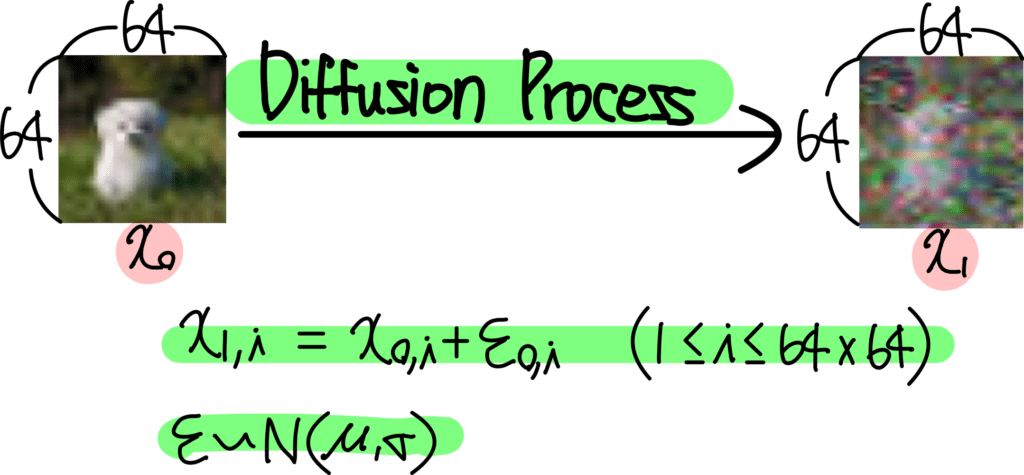
Diffusion Model에 관한 설명 및 수식은 위의 블로그들을 참고했다.

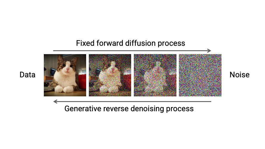
Forward Diffusion Process를 통해 매 time step마다 Input Image의 모든 pixel에 Gaussian Noise $\varepsilon_{\theta}$를 추가하고,

Reverse Denoising Process를 통해 매 time step마다 추가된 Gaussian Noise $\varepsilon_{\theta}$를 제거함으로써,

Input Image와 유사한 확률분포를 가지는 Result Image를 생성하는 모델이다.

Input Image에서 Gaussian Noise가 서서히 확산되기에 Diffusion(확산)이라는 이름이 붙었다고 한다.

• Forward Diffusion Process: Input Image에 fixed(고정된) Gaussian Noise가 더해진다.
• Reverse Denoising Process: Result Image에 learned(학습된) Gaussian Noise가 빼진다.

Diffusion Model의 목적은

Forward Diffusion Process를 거친 Result Image의 확률분포를 Reverse Denoising Process를 통해 Input(Real) Image의 확률분포와 유사하게 만드는 것이다.

이를 달성하기 위해 Reverse Denoising Process에서 학습을 통해 Noise 생성 확률 분포 Parameter인 Mean $\mu$, Standard Deviation $\sigma$를 조절한다.

1. Diffusion Basics

"Diffusion"이라 함은 "확산" 현상을 의미한다.

아래의 그림을 보면 지정된 space안의 공기 분자들이 시간이 지남에 따라 Diffusion Process를 통해 전체 space안에 고르게 분포하는 것을 알 수 있다.

이때, 공기 분자 하나의 움직임을 관찰해보자.

매우 짧은 time step (sequence)동안 하나의 분자가 움직이는 Movement는 Gaussian Distribution을 따른다.

위의 그림은 매우 짧은 time step $t$ 단위로 분자 하나의 Movement $m_{t}$ 를 표시한 것이다. 이때, Movement $m_{t}$는 Gaussian Distribution을 따르므로 $m_{t} \sim N(\mu, \sigma)$으로 표현가능하다.

즉, 매시간 $t$마다 각 분자들은 Gaussian Distribution에 의한 Movement를 수행하는데 만약 이 Movement들을 예측해낼 수 있다면 Reverse Diffusion Process에 의해 Noisy 하지 않은 원상태를 구현할 수 있다.

이제, 위의 Diffusion Process를 Image에 적용해보자.

매 time step $t$마다 Molcule(분자)에 Gaussian Distribution을 따르는 Noise Movement $m_{t}$ 가 더해져 최종 Movement가 결정된다. 반면에 Image에서는 각 pixel에 Gaussian Noise $\varepsilon_{\theta}$ 가 더해져 그 다음 time step의 pixel이 된다.

위의 내용들을 종합하여 수식으로 나타내면 다음과 같다:

• $x_{0}$: 원본 image ($N \times N$ size)
• $x_{1}$: 다음 time step의 image
• $i$: image에 위치한 pixel의 position (index)

이미지의 각 pixel position에 대해 다음과 같이 식이 작성된다.

$x_{1, i}$ = $x_{0, i} + \varepsilon_{o, i}$ ($1 \leq i \leq N^{2}$)

$\varepsilon \sim N(\mu, \sigma)$

위의 예시는 $64 \times 64$의 image의 모든 pixel value에 Gaussian Noise $\varepsilon_{\theta}(x_{t}, t)$을 추가해주는 과정이다.

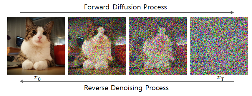
이러한 과정을 수많은 time step $t$ 마다 반복하여 완전한 Noise Image로 만들어준다. 이는 아래의 그림을 통해 설명가능하다.

위 과정은 Diffusion Forward Process라 한다. 매 time step $t$ 마다 이전 이미지 $x_{t-1}$의 모든 pixel에 fixed Gaussian Noise $\varepsilon$를 추가하여 time step $t$ 에서의 이미지 $x_{t}$를 형성한다.

위의 과정을 반복하여 최종 time step $T$에서는 $x_{T}$가 완전한 Noise Image가 되어있음을 알 수 있다.

이때, 매 time step $t$에서 첨가된 Gaussian Noise $\varepsilon_{\theta}(x_{t}, t)$을 계산할 수 있다면 Noise Image $x_{T}$에서 Real Image (Data) $x_{0}$로 Noise를 제거하면서(Subtraction) 되돌리는 것이 가능하다.

이는 Image Generation이 가능하다는 말을 뜻한다.

• Input: $x_{T}$ (random noise image)
• Output: $x_{0}$ (real / desired image)
• Process: Reverse Diffusion Process

정리해보면, Diffusion Model은 time step $t$에서의 image $x_{t}$를 입력으로 받아, 각 pixel별로 추가된 Gaussian Noise $\varepsilon_{\theta}(x_{t}, t)$를 예측하는 것이다.

해당 Noise $\varepsilon$를 subtract하면 이전 time step $t-1$에서의 image (less noisy image)로 변환가능하기에, $x_{T}$에서 위의 과정을 반복해 나가면 결국 real image (Data) $x_{0}$를 구현해낼 수 있다.

Diffusion Model이 갖춰야 하는 4가지 Condition들은 다음과 같다:

1. Input: Image or Noisy Image (3D Tensor 형태 or 2D Array 형태여야 한다)
2. Time step: 몇 번째 Process인지를 의미하는 $t$도 주어져야 한다.
3. Condition: 추가 Condition이 있다면 이 조건 또한 Diffusion Model에 주어져야 한다.
   1. Condition이란 특정 class 정보, 또는 생성한 이미지를 표현할 Text 정보 등등이 해당한다.
   2. Classifier Guidance를 통해 주어질 수도 있고, 바로 Diffusion Model에 주어질 수도 있다.
4. Output: Input과 동일한 Shape여야 한다.
   1. value는 각 pixel별로 첨가된 Noise값을 의미한다.
   2. Diffusion Model에 따라 Noise값 자체를 예측할지, Noise의 $\mu, \sigma$등을 예측할지는 조금씩 다르지만, Noise를 예측한다고 이해하면 큰 문제는 없다.

위 그림은 일반적인 Diffusion Model의 Architecture를 표현한 그림인데, Diffusion Model은 U-Net 구조를 띄고 있는 것을 알 수 있다.

• U-Net의 Structure 특성상 이는 Input과 동일한 Resoution을 가지는 Output을 내기에 용이하다.
• time step $t$ 를 별도로 입력받는다.
• 위의 구조는 대부분의 Diffusion Model에서 공통적으로 사용되고 있는 구조다.

앞서 말했듯, Diffusion Model은 time step $t$에서

• Input: Noisy Image $x_{t}$
• Output: Gaussian Noise $\varepsilon_{\theta}(x_{t}, t)$

위와 같음을 알 수 있다.

따라서, 각 pixel마다 첨가된 Gaussian Noise $\varepsilon_{\theta}$을 예측하는데, Loss Function은 아래와 같이 표현가능하다.

• $\varepsilon$: Ground Truth (Real Noise)
• $\varepsilon_{\theta}$: Diffusion Model이 예측한 Noise

위의 두 항이 같아지도록 Diffusion Model을 학습시킨다.

2. Diffusion Process

최근 Diffusion Model이 GAN을 압도하는 Score를 내면서 새롭게 Generative Model의 새로운 강자로 떠오르고 있다.

Physical Intuition

매우 작은 time step이나 sequence에서는 Diffusion Model의 forward/backward process 모두 Gaussian Noise의 addition/subtraction 으로 볼 수 있다.

• Forward Diffusion Process: Input Image $x_{0}$에 Noise를 점진적으로 더한다
• Reverse Denoising Process: Denoising을 통해 $x_{T}$에서 $x_{0}$로 data generation을 수행한다.

현재 상태($\mathbf{x}_{t}$)는 이전 상태($\mathbf{x}_{t-1}$)에 의존한다는 마르코프(Markov) 특성을 가진다.

이전 상태($\mathbf{x}_{t-1}$)가 주어질 때 현재 상태($\mathbf{x}_{t}$)가 될 확률분포 $q(\mathbf{x}_{t}|\mathbf{x}_{t-1})$는 평균($\mu$)과 분산($\Sigma$)으로 구성된 Gaussian Distribution(=$N$= Normal Distribution)을 따른다.

Forward Diffusion Process

이 식을 Noise Injection parameter인 $\beta_{t}$(fixed)를 포함하여 다르게 표현하면, 이전 상태($\mathbf{x}_{t-1}$)의 이미지가 $\beta_{t}$만큼 다른 pixel을 선택하게 하고, $\sqrt{1-\beta_{t}}$ 만큼 이전 pixel값을 선택하게 하는 식으로 정의 할 수 있다.

$t$가 점점 증가함에 따라 $\beta_{t}$가 커짐으로써 Noise가 강해진다.

Forward과정에서 $\beta_{t}$는 각 time step에서 Injection되는 Noise가 고정(fixed)되어 있지만, 확률 분포를 따르기 때문에 마지막 상태($\mathbf{x}_{T}$)의 결과가 항상 다를 수 있다.

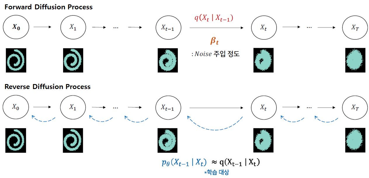
• $q(\mathbf{x}_{t}|\mathbf{x}_{t-1})$: 이전 상태($x_{t-1}$) 주어졌을 때 현재 상태($x_{t}$)가 될 확률분포
• $q(\mathbf{x}_{t-1}|\mathbf{x}_{t})$: 현재 상태($x_{t}$) 주어졌을 때 이전 상태($x_{t-1}$)가 될 확률분포

Reverse Denoising Process

다음으로 Reverse과정에서 마지막 상태($\mathbf{x}_{T}$)를 반대로 최초 상태($\mathbf{x}_{0}$)로 만들고자 한다.

$q(\mathbf{x}_{t}|\mathbf{x}_{t-1})$식의 좌항(posterior)과 우측항(prior)을 바꾼 조건부 확률 $q(\mathbf{x}_{t-1} | \mathbf{x}_{t})$을 알 수 있다면, 최초 상태($\mathbf{x}_{0}$)로 만들 수 있겠지만 이를 계산 할 수가 없다.

각 $t$ 시점에서 이미지의 확률 분포$q(\mathbf{x}_{t})$를 알 수 없기 때문에 베이즈 정리에 의해 계산되지 않는다.

때문에 확률분포 $q$가 주어졌을 때, 이 확률 분포를 가장 잘 모델링하는 확률 분포 $p_{θ}$를 찾는 문제로 변환한다.

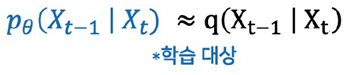
즉 확률분포 $q$에서 관측한 값으로 확률 분포 $p_{\theta}$의 likelihood를 구하였을 때,
그 likelihood값이 최대(Maximum)가 되는 확률분포를 찾는 Maximum Likelihood Estimation(MLE) 문제다.

Forward Diffusion Process는 다음과 같이 이루어진다.

• Image (Data)에서 Noise로 이동하는 Process
• $q(\textbf{x}_{t}|\textbf{x}_{t-1}) = N(\mathbf{x}_t ; \mu_{\mathbf{x}_t}, \Sigma_{\mathbf{x}_t} ) = N(\textbf{x}_{t}; \sqrt{1-\beta_{t}} \textbf{x}_{t-1}, \beta_{t}\textbf{I})$
  • $q(\textbf{x}_{t}|\textbf{x}_{t-1})$: 이전 상태 $x_{t-1}$가 주어졌을 때, 현재 상태 $x_{t}$가 나올 확률분포
  • $\textbf{x}_{t}$: Random Variable (확률변수)
  • $\sqrt{1-\beta_{t}} \textbf{x}_{t-1}$: Mean (평균)
  • $\beta_{t}\textbf{I}$: Covariance Matrix (공분산 행렬)
  • $\sqrt{\beta_{t}}\textbf{I}$: Standard Deviation ($\sqrt{ }$를 씌워야 한다)

Forward Diffusion Process

$$q(\textbf{x}_{1:T} | \textbf{x}_{0}) = \prod_{t=1}^{T} q(\textbf{x}_{t}|\textbf{x}_{t-1})$$

$N(\textbf{x}_{t}; \sqrt{1-\beta_{t}} \textbf{x}_{t-1}, \beta_{t}\textbf{I})$와 같이 설정한 이유는 $Var(\mathbf{x}_{t-1})=\mathbf{I}$이라고 가정했을 때, $Var(\mathbf{x}_{t})=\mathbf{I}$으로 맞춰주기 위해서이다.

$$\mathbf{x}_t = \sqrt{1-\beta_t}\mathbf{x}_{t-1} + \sqrt{\beta_t}\boldsymbol{\epsilon}, \quad \boldsymbol{\epsilon} \sim \mathcal{N}(0, \mathbf{I})$$

- $\text{Var}(\varepsilon) = \mathbf{I}$

- $\mathbf{x}_{t}$는 Gaussian Distribution에서 sampling했기 때문에 Covariance Matrix의 각 element인 $\beta_{t}$에 $\varepsilon$를 곱하면 된다.

- Identity Matrix $I$를 $\varepsilon$에 곱하는 것이 아니라 $\mathbf{x}_{t}$를 sampling했기에 standard deviation value $\sqrt{\beta_{t}}$를 가지고 $\varepsilon$에 바로 곱해주면 된다.

매 time step $t$마다 조금씩 Gaussian Noise를 더한다면, 결국 Gaussian Kernel이 연속적이기 때문에 Joint Distribution을 통해 하나의 time step에 대한 식으로 한번에 정리가능하다.

• Diffusion Kernel: $q(\mathbf{x}_t|\mathbf{x}_0) = \mathcal{N}(\mathbf{x}_t; \sqrt{\bar{\alpha}_t}\mathbf{x}_0, (1 - \bar{\alpha}_t)\mathbf{I})$
  • $q(\mathbf{x}_{t}|\mathbf{x}_{0})$: 최초 상태($x_{0}$)가 주어졌을 경우, 특정 시점의 상태($x_{t}$)가 나올 확률분포에 대한 식
• For Sampling: $\mathbf{x}_t = \sqrt{\bar{\alpha}_t} \mathbf{x}_0 + \sqrt{(1 - \bar{\alpha}_t)} \epsilon \quad \text{where} \quad \epsilon \sim \mathcal{N}(0, \mathbf{I})$
  • $\alpha_t = 1 - \beta_t$ and $\bar{\alpha}_{t} = \prod_{s=1}^{t} \alpha_s$
  • 특정 시점의 상태($x_{t}$)를 구하는데 있어서, 최초 상태($x_{0}$)에서 바로 Define할 수 있다.
  • $x_{0}$에서의 이미지만 있다면 time step $T$에서의 noisy image를 바로 구할 수 있다는 의미이다.

왜 갑자기 위의 식이 도출되는지에 대해 의문이 든다면, 아래의 "Forward Diffusion Process: $q(\mathbf{x}_{t}|\mathbf{x}_{0})$" Callout Block을 참고하길 바란다.

결국 매 time step $t$마다 gaussian noise를 추가해서 최종적으로 gaussian distribution에 가까운 $q(\mathbf{x}_{T})$를 얻는 process이다.

$$q(\mathbf{x}_t) = \int q(\mathbf{x}_0, \mathbf{x}_t) d\mathbf{x}_0 = \int q(\mathbf{x}_0) q(\mathbf{x}_t|\mathbf{x}_0) d\mathbf{x}_0$$

위의 식을 보면 알 수 있듯이,

$$\text{We can sample } \mathbf{x}_t \sim q(\mathbf{x}_t) \text{ by first sampling } \mathbf{x}_0 \sim q(\mathbf{x}_0) \text{ and then sampling } \mathbf{x}_t \sim q(\mathbf{x}_t|\mathbf{x}_0) \text{ (i.e., ancestral sampling).}$$

각각 sampling을 통해 최종 time step $T$에서의 probability distribution을 구할 수 있다.

Reverse Denoising Process의 목적은 Noisy Image $\mathbf{x}_{T}$에서 다시 원본 Data (Real Image) $\mathbf{x}_{0}$의 확률분포와 유사하게 만드는 것이다.

Physical Intuition에 의해, Reverse Step 또한 마찬가지로 각 Probability Distribution $q(\mathbf{x}_{t-1}|\mathbf{x}_{t})$이 Gaussian Process라고 볼 수 있다.

Gaussian Noise로부터 시작을 해서,

$$p(\mathbf{x}_T) = \mathcal{N}(\mathbf{x}_T; 0, \mathbf{I})$$

확률분포 $q$가 주어졌을 때, 이 확률 분포를 가장 잘 모델링하는 확률 분포 $p_{θ}$를 찾는다.

$$p_{\theta}(\mathbf{x}_{t-1}|\mathbf{x}_{t}) = \mathcal{N}(\mathbf{x}_{t-1}; \mu_{\theta}(\mathbf{x}_t, t), \Sigma_{\theta}(\mathbf{x}_{t}, t))$$

가 되는데, 이때

• $ \mu_{\theta}(\mathbf{x}_t, t)$: Mean
• $\Sigma_{\theta}(\mathbf{x}_{t}, t)$: Variance

두 개의 파라미터를 어떻게 Train시킬지가 굉장히 중요해진다.

Reverse Denoising Process

$$p_{\theta}(\mathbf{x}_{0:T}) = p(\mathbf{x}_{T})\prod_{t=1}^{T} p_{\theta}(\mathbf{x}_{t-1}|\mathbf{x}_{t})$$

위와 같이 probability distribution들의 joint의 형태로 표현이 가능하다.

• $q(\textbf{x}_{1:T} | \textbf{x}_{0}) = \prod_{t=1}^{T} q(\textbf{x}_{t}|\textbf{x}_{t-1})$: Forward Diffusion Process
• $p_{\theta}(\mathbf{x}_{0:T}) = p(\mathbf{x}_{T})\prod_{t=1}^{T} p_{\theta}(\mathbf{x}_{t-1}|\mathbf{x}_{t})$: Reverse Denoising Process

3. Learning Diffusion Model

$ \mu_{\theta}(\mathbf{x}_t, t)$의 Mean, $\Sigma_{\theta}(\mathbf{x}_{t}, t)$의 Variance는 어떻게 Train 시켜야 하는가?

Variational Upper Bound를 사용한다.

• Foward Diffusion Process: $q(\mathbf{x}_{t}|\mathbf{x}_{t-1}, \mathbf{x}_{0})$
• Reverse Denoising Process: $p_{\theta}(\mathbf{x}_{t-1}|\mathbf{x}_{t})$

$$\mathbb{E}{q(x_0)}[-\log p_{\theta}(\mathbf{x}_{0})] \leq \mathbb{E}_{q(x_{0})q(x_{1:T}|x_{0})}\left[-\log \frac{p_\theta(x_{0:T})}{q(x_{1:T}|x_{0})}\right] =: L$$

variational upper bound를 사용하는데, 이를 통해 아래의 Loss Term을 만든다.

$$L = \mathbb{E}q\left[D_{\text{KL}}(q(\mathbf{x}_{T}|\mathbf{x}0)||p(\mathbf{x}_{T})) + \sum_{t>1}D_{\text{KL}}(q(\mathbf{x}_{t-1}|\mathbf{x}_{t}, \mathbf{x}_{0})||p_{\theta}(\mathbf{x}_{t-1}|\mathbf{x}_{t})) - \log p_{\theta}(\mathbf{x}_{0}|\mathbf{x}_{1})\right]$$

위의 Loss를 최소화시켜서 평균을 구하는 것을 목표로 하는데, 이는 일종의 Regression과 비슷하다고 볼 수 있다.

• $L_{T}$: Noise Injection Parameter $\beta$가 fix되어 학습이 되지 않아 제거된다.
• $q(\mathbf{x}_{t-1}|\mathbf{x}_{t}, \mathbf{x}_{0})$는 tractable posterior distribution으로, 아래와 같이 Gaussian Distribution으로 처리 가능하다.

$$q(\mathbf{x}_{t-1}|\mathbf{x}_t,\mathbf{x}_0) = \mathcal{N}(\mathbf{x}_{t-1}; \tilde{\mu}_t(\mathbf{x}_t,\mathbf{x}_0), \tilde{\beta}_t I)$$

$$\tilde{\mu}_t(\mathbf{x}_t,\mathbf{x}_0) := \frac{\sqrt{\bar{\alpha}_{t-1}}\beta_t}{1-\bar{\alpha}_t}\mathbf{x}_0 + \frac{\sqrt{1-\bar{\beta}_t}(1-\bar{\alpha} _{t-1})}{1-\bar{\alpha}_t}\mathbf{x}_t \quad \text{and} \quad \tilde{\beta}_t := \frac{1-\bar{\alpha}_{t-1}}{1-\bar{\alpha}_t}\beta_t$$

$q(\mathbf{x}_{t-1}|\mathbf{x}_{t}, \mathbf{x}_{0})$와 $p_{\theta}(\mathbf{x}_{t-1}|\mathbf{x}_{t})$ 모두 Gaussian Distribution으로 가정을 했으므로 그에 관한 공식을 이용한다.

이때, 앞의 Forward Diffusion Process에서 언급한 Reparameterization Trick을 이용한 결과를 이용하자.

$$\mathbf{x}_t = \sqrt{\bar{\alpha}_t} \mathbf{x}_0 + \sqrt{(1-\bar{\alpha}_t)} \epsilon$$

이므로, 이 식을 이용하면 $\tilde{\mu}_t(\mathbf{x}_t, \mathbf{x}_0)$는 다음과 같이 표현가능하다.

$$\tilde{\mu}_t(\mathbf{x}_t, \mathbf{x}_0) = \frac{1}{\sqrt{1-\beta_t}}\left(\mathbf{x}_t - \frac{\beta_t}{\sqrt{1-\bar{\alpha}_t}}\epsilon\right)$$

최종적으로 알고 싶은 것은, Reverse Denoising Process에서의 Gaussian Noise의 Mean이므로 다음과 같이 표현된다.

Noise-Prediction Network에 의해 평균 $\mu_\theta(\mathbf{x}_t, t)$을 예측할 수 있다.

$$\mu_\theta(\mathbf{x}_t, t) = \frac{1}{\sqrt{1-\beta_t}}\left(\mathbf{x}_t - \frac{\beta_t}{\sqrt{1-\bar{\alpha}_t}}\epsilon_\theta(\mathbf{x}_t, t)\right)$$

결과적으로, 수식을 보면 Train되는 Gaussian Noise의 Mean은 Noise Prediction의 $\epsilon_\theta(\mathbf{x}_t, t)$만 구하면 예측가능하다.

최종적으로 $L_{t-1}$의 식을 $\mathbf{x}_{t}$를 대입해서 정리해보면 다음과 같다.

$$L_{t-1} = \mathbb{E}_{\mathbf{x}_0 \sim q(\mathbf{x}_0), \epsilon \sim \mathcal{N}(0,\mathbf{I})}\left[\frac{\beta_t^2}{2\sigma_t^2(1-\beta_t)(1-\bar{\alpha}_t)}||\epsilon - \epsilon_\theta(\sqrt{\bar{\alpha}_t} \mathbf{x}_0 + \sqrt{1-\bar{\alpha}_t} \epsilon, t)||^2\right] + C$$

이때, $||\tilde{\mu}_{t}(\mathbf{x}_t, \mathbf{x}_0) - \mu_{\theta}(\mathbf{x}_t, t)||^2$ 앞에 있는 여러 Coefficient들을 $1$로 간단하게 처리하는게 학습이 잘된다고 DDPM Paper에서 주장한다.

Advanced Weighting에 부분에 있는 논문들은 $1$이 아닌 다른 값들을 사용하자고 주장하는 논문들이다.

• 1) Training: Loss를 학습시켜서 Noise를 예측하는 Network를 학습
• 2) Sampling: 수식적으로 도출된 Mean, Variance를 기반으로 Sampling을 진행
• time step $1 \sim T$을 보통 1000번 정도 설정한다

여기서 Algorithm2의 Sampling 부분의 빨간색 박스는 아래와 같이 이해할 수 있다.

$$\mathbf{x}_{t-1} = \mu_\theta(\mathbf{x}_t, t) + \sigma_t \mathbf{z}$$

$$= \frac{1}{\sqrt{\alpha_t}} \left(\mathbf{x}_t - \frac{1-\alpha_t}{\sqrt{1-\bar{\alpha}_t}} \epsilon_\theta (\mathbf{x}_t, t)\right) + \sigma_t \mathbf{z}$$

• $\mathbf{x}_{0} \sim q(\mathbf{x}_{0})$, $t \sim \text{Uniform}({1, ... , T})$, $\varepsilon \sim \mathcal{N}(o, \mathbf{I})$에서 각각 Sample
• $\mathbf{x}_{t}$: $\mathbf{x}_t = \sqrt{\bar{\alpha}_t} \mathbf{x}_0 + \sqrt{(1 - \bar{\alpha}_t)} \epsilon \quad \text{where} \quad \epsilon \sim \mathcal{N}(0, \mathbf{I})$를 이용해서 Real Image $\mathbf{x}_0 $으로부터 한번에 얻는다.
  • 한 번에 구하지 않을 경우 $t=0$부터 지정한 time step $t$까지 Gaussian Kernel을 $t+1$개 생성해야 하므로 cost가 늘어난다.
• $t$: Sin, Cos를 이용한 Positional Encoding을 한 후에 FC Layer (Linear Embedding)를 통과하여 U-Net의 모든 Layer에 Projection 시켜준다.
• Output: Noise $\varepsilon_{\theta}(\mathbf{x}_{t}, t)$ 를 예측한다.

• Forward Process | $\beta_{t}$: Noise Injection Parameter
  • Linear하게 설정하거나 Paper 나름대로 여러 방식을 사용
  • 0.005부터 시작해서 0에 가까워지도록 일반적으로 설정
• Reverse Process | $\sigma_{t}^{2}$: Variance Term
  • DDPM에서는 $\sigma_{t}^{2} = \beta_{t}$으로 설정
  • 아래 첨부한 Paper들은 다른 방식을 주장

Reverse Denoising Process를 수행할 때, U-Net이 time step $t$에 따라 담당하는 구간이 다르다.

• $\mathbf{x}_{T}$ 근처 time step: Low-Frequency Content, coarse content
• $\mathbf{x}_{0}$ 근처 time step: High-Frequency Content, low-level details

4. DDPM Formulas

현재 상태($\mathbf{x}_{t}$)는 오직 이전 상태($\mathbf{x}_{t-1}$)에만 의존한다는 Markov 특성을 지닌다.

$$q(\mathbf{x}_T|\mathbf{x}_{T-1}) = q(\mathbf{x}_T|\mathbf{x}_{T-1}, \mathbf{x}_{T-2}, ..., \mathbf{x}_1, \mathbf{x}_0)$$

즉, 위의 식이 성립하기에 아래와 같이 식변형이 가능하다.

$$\quad q(\mathbf{x}_{1:T}|\mathbf{x}_0) = \prod _{t=1}^T q(\mathbf{x}_t|\mathbf{x}_{t-1}) = q(\mathbf{x}_1|\mathbf{x}_0)q(\mathbf{x}_2|\mathbf{x}_1)q(\mathbf{x}_3|\mathbf{x}_2)...q(\mathbf{x}_T|\mathbf{x}_{T-1}) $$

$$= q(\mathbf{x}_1|\mathbf{x}_0)q(\mathbf{x}_2|\mathbf{x}_1, \mathbf{x}_0)q(\mathbf{x}_3|\mathbf{x}_2, \mathbf{x}_1, \mathbf{x}_0)...q(\mathbf{x}_T|\mathbf{x}_{T-1}, .... , \mathbf{x}_1, \mathbf{x}_0)$$

$$= \frac{q(\mathbf{x}_1,\mathbf{x}_0)}{q(\mathbf{x}_0)} \frac{q(\mathbf{x}_2,\mathbf{x}_1,\mathbf{x}_0)}{q(\mathbf{x}_1,\mathbf{x}_0)}...\frac{q(\mathbf{x}_T,\mathbf{x}_{T-1},...,\mathbf{x}_1,\mathbf{x}_0)} {q(\mathbf{x}_{T-1},...,\mathbf{x}_0)}$$

$$= \frac{q(\mathbf{x}_0,\mathbf{x}_1,\mathbf{x}_2,\mathbf{x}_3,...,\mathbf{x}_T)}{q(\mathbf{x}_0)} = \quad q(\mathbf{x}_{1:T}|\mathbf{x}_0)$$

$$q(\textbf{x}_{1:T} | \textbf{x}_{0}) = \prod_{t=1}^{T} q(\textbf{x}_{t}|\textbf{x}_{t-1})$$

$q(\mathbf{x}_t | \mathbf{x}_{0})$: 최초 상태($x_{0}$)가 주어졌을 경우, 특정 시점의 상태($x_{t}$)가 나올 확률분포에 대한 식이다.

$q(\mathbf{x}_t | \mathbf{x}_{t-1})$는 다음과 같이 정의가능하다.

$q(\mathbf{x}_t | \mathbf{x}_{t-1}) := N(\mathbf{x}_t ; \mu_{\mathbf{x}_{t-1}}, \Sigma_{\mathbf{x}_{t-1}}) := N(\mathbf{x}_t ; \sqrt{1-\beta_t} \mathbf{x}_{t-1}, \beta_t I)$

이때, $\alpha_t = 1 - \beta_t$ and $\bar{\alpha}_{t} = \prod_{s=1}^{t} \alpha_s$라 한다면,

$X$가 Gaussian Distribution을 따를 때, 아래의 Reparameterization Trick을 사용할 수 있다.

따라서, $\mathbf{x}_{t}$는 다음과 같이 정의할 수 있다.

$\mathbf{x}_{t} = \sqrt{\alpha_{t}}\mathbf{x}_{t-1} + \sqrt{1-\alpha_{t}}\epsilon_{t-1} \quad \text{;where } \epsilon_{t-1}, \epsilon_{t-2}, \cdots \sim \mathcal{N}(0, \mathbf{I})$

이제 $\mathbf{x}_{t-1}$의 자리에 순서대로 역대입을 하여 계산을 하면,

$\mathbf{x}_{t} = \sqrt{\alpha_t}\mathbf{x}_{t-1} + \sqrt{1-\alpha_{t}}\epsilon_{t-1} \quad \text{;where } \epsilon_{t-1}, \epsilon_{t-2}, \cdots \sim \mathcal{N}(0, \mathbf{I})$

$= \sqrt{\alpha_t\alpha_{t-1}}\mathbf{x}_{t-2} + \sqrt{1-\alpha_t\alpha_{t-1}}\epsilon_{t-2} \quad \text{;where } \epsilon_{t-2} \text{ merges two Gaussians (*).}$

$= \cdots$

$= \sqrt{\bar{\alpha}_t}\mathbf{x}_0 + \sqrt{1-\bar{\alpha}_t}\epsilon$

위와 같이 정리할 수 있으며,

결과적으로 아래와 같은 식을 도출할 수 있다.

$q(\mathbf{x}_t|\mathbf{x}_0) = \mathcal{N}(\mathbf{x}_t; \sqrt{\bar{\alpha}_t}\mathbf{x}_0, (1 - \bar{\alpha}_t)\mathbf{I})$

두 개의 Gaussian Noise를 합칠 때 왜 식이 저렇게 되는지에 대해 의문이 든다면 아래의 toggle을 확인해보길 바란다.

그렇다면 왜 아래의 식이 성립할까?

$$\sqrt{\alpha_{t}(1-\alpha_{t-1})}\epsilon_{t-2} + \sqrt{1-\alpha_{t}}\epsilon_{t-1} = \sqrt{\alpha_{t}(1-\alpha_{t-1}) + (1-\alpha_{t})}\tilde{\epsilon}_{t-2}$$

그건 Gaussian Distribution의 Linearity에 관한 특성 때문이다.

$$p_{\theta}(\mathbf{x}_{0:T}) = p(\mathbf{x}_{T})\prod_{t=1}^{T} p_{\theta}(\mathbf{x}_{t-1}|\mathbf{x}_{t})$$

Markov Chain에 의해 다음의 식이 성립한다:

$$p_\theta(x_0|x_1)p_\theta(x_1|x_2)p_\theta(x_2|x_3)...p_\theta(x_{T-1}|x_T)$$

$$= p_\theta(x_0|x_1,..., x_{T-1}, x_T)p_\theta(x_1 |x_2, ..., x_{T-1}, x_T)...p_\theta(x_{T-1}|x_T)$$

$$ = \frac{p_\theta(x_0,x_1,...,x_{T-1},x_T)}{p_\theta(x_1,...,x_{T-1},x_T)} \frac{p_\theta(x_1,...,x_{T-1},x_T)}{p_\theta(x_2,...,x_{T-1},x_T)}...\frac{p_\theta(x_{T-1},x_T)}{p_\theta(x_T)}$$

$$= \frac{p_\theta(x_0,x_1,...,x_{T-1},x_T)} {p_\theta(x_T)} = \frac{p_{\theta}(\mathbf{x}_{0:T})} {p_\theta(x_T)}$$

Forward Process: time step $t=0$에서 $t=T$로 갈수록 과거에서 미래로 간다고 해석한다.


Reverse Process: time step $t=T$에서 $t=0$로 갈수록 과거에서 미래로 간다고 해석한다.


따라서 Markov Chain의 성질을 적용할 때 주어진 Condition을 추가해도 되는 경우는 과거 의 경우에 한정하므로 Forward인지, Reverse인지 잘 구분해야 한다.

그렇다면 왜 DDPM의 Loss가 저런 형태를 띄는지에 대해 알아볼 필요가 있다.

우선, Variational AutoEncoder인 VAE의 Variational Upper Bound에서 시작한다.

$$\mathbb{E}_{x_T \sim q(x_T|x_0)}[-\log p_\theta(x_0)]$$

1) $$= \mathbb{E}_{x_T \sim q(x_T|x_0)}\left[-\log \frac{p_\theta(x_0, x_1, x_2, ..., x_T)}{p_\theta(x_1, x_2, x_3, ..., x_T|x_0)}\right] \quad \because \text{bayes rule}, p_\theta(x_T|x_0) = \frac{p_\theta(x_T, x_0)}{p_\theta(x_0)}$$

2) $$= \mathbb{E}_{x_T \sim q(x_T|x_0)}\left[-\log \frac{p_\theta(x_0, x_1, x_2, ..., x_T)}{p_\theta(x_1, x_2, x_3, ..., x_T|x_0)} \cdot \frac{q(x_{1:T}|x_0)}{q(x_{1:T}|x_0)}\right]$$

3) $$\leq \mathbb{E}_{x_T \sim q(x_T|x_0)}\left[-\log \frac{p_\theta(x_0, x_1, x_2, ..., x_T)}{q(x_{1:T}|x_0)}\right] \quad \because \text{KL divergence} > 0, \text{"ELBO"}$$

4) $$= \mathbb{E}_{x_T \sim q(x_T|x_0)}\left[-\log \frac{p_\theta(x_{0:T})}{q(x_{1:T}|x_0)}\right] \quad \because \text{Notation}$$

5) $$= \mathbb{E}_{x_T \sim q(x_T|x_0)}\left[-\log \frac{p_\theta(x_T) \prod_{t=1}^T p_\theta(x_{t-1}|x_t)}{\prod_{t=1}^T q(x_t|x_{t-1})}\right] \quad \because \text{Below Markov chain property}$$

6) $$= \mathbb{E}_{x{1:T} \sim q(x_{1:T}|x_0)}\left[-\log p_\theta(x_T) - \sum_{t=1}^T \log \frac{p_\theta(x_{t-1}|x_t)}{q(x_t|x_{t-1})}\right] \quad \because \text{separating to summation in logarithm}$$

$$p_\theta(x_{0:T}) := p_\theta(x_T) \prod_{t=1}^T p_\theta(x_{t-1}|x_t) \qquad q(x_{1:T}|x_0) := \prod_{t=1}^T q(x_t|x_{t-1})$$

7) $$= \mathbb{E}_{x{1:T} \sim q(x_{1:T}|x_0)}\left[-\log p_\theta(x_T) - \sum_{t=1}^T \log \frac{p_\theta(x_{t-1}|x_t)}{q(x_t|x_{t-1})}\right]$$

8) $$= \mathbb{E}_{x{1:T} \sim q(x_{1:T}|x_0)}\left[-\log p_\theta(x_T) - \sum_{t=2}^T \log \frac{p_\theta(x_{t-1}|x_t)}{q(x_t|x_{t-1})} - \log \frac{p_\theta(x_0|x_1)}{q(x_1|x_0)}\right]$$

9) $$= \mathbb{E}_{x{1:T} \sim q(x_{1:T}|x_0)}\left[-\log p_\theta(x_T) - \sum_{t=2}^T \log \frac{p_\theta(x_{t-1}|x_t)}{q(x_{t-1}|x_t, x_0)} \cdot \frac{q(x_{t-1}|x_0)}{q(x_t|x_0)} - \log \frac{p_\theta(x_0|x_1)}{q(x_1|x_0)}\right] \quad \because *$$

$$q(x_t|x_{t-1}) = q(x_t|x_{t-1}, x_0) \quad \because \text{Markov chain property}$$

$$= \frac{q(x_t, x_{t-1}, x_0)}{q(x_{t-1}, x_0)} \quad \because \text{bayes rule}$$

$$= \frac{q(x_{t-1}, x_t, x_0)}{q(x_{t-1}, x_0)} \cdot \frac{q(x_t, x_0)}{q(x_t, x_0)}$$

$$= q(x_{t-1}|x_t, x_0) \cdot \frac{q(x_t, x_0)}{q(x_{t-1}, x_0)}$$

10) $$= \mathbb{E}_{x{1:T} \sim q(x_{1:T}|x_0)}\left[-\log p_\theta(x_T) - \sum_{t=2}^T \log \frac{p_\theta(x_{t-1}|x_t)}{q(x_{t-1}|x_t, x_0)} - \sum_{t=2}^T \log \frac{q(x_{t-1}|x_0)}{q(x_t|x_0)} - \log \frac{p_\theta(x_0|x_1)}{q(x_1|x_0)}\right]$$

11) $$= \mathbb{E}_{x{1:T} \sim q(x_{1:T}|x_0)}\left[-\log p_\theta(x_T) - \sum_{t=2}^T \log \frac{p_\theta(x_{t-1}|x_t)}{q(x_{t-1}|x_t, x_0)} - \log \frac{q(x_1|x_0)}{q(x_T|x_0)} - \log \frac{p_\theta(x_0|x_1)}{q(x_1|x_0)}\right]$$

12) $$= \mathbb{E}_{x{1:T} \sim q(x_{1:T}|x_0)}\left[-\log \frac{p_\theta(x_T)}{q(x_T|x_0)} - \sum_{t=2}^T \log \frac{p_\theta(x_{t-1}|x_t)}{q(x_{t-1}|x_t, x_0)} - \log p_\theta(x_0|x_1)\right]$$

따라서 최종 DDPM Loss는 아래와 같이 정리할 수 있다.

$$L = \mathbb{E}_q\left[D_\text{KL}(q(x_T|x_0)||p(x_T)) + \sum_{t>1} D_\text{KL}(q(x_{t-1}|x_t, x_0)||p_\theta(x_{t-1}|x_t)) - \log p_\theta(x_0|x_1)\right]$$

$q(\mathbf{x}_{t-1}|\mathbf{x}_{t}, \mathbf{x}_{0})$이 아래와 같이 표현가능한 이유를 수식적으로 알아보자.

$$q(\mathbf{x}_{t-1}|\mathbf{x}_t,\mathbf{x}_0) = \mathcal{N}(\mathbf{x}_{t-1}; \tilde{\mu}_t(\mathbf{x}_t,\mathbf{x}_0), \tilde{\beta}_t I)$$

$$\tilde{\mu}_t(\mathbf{x}_t,\mathbf{x}_0) := \frac{\sqrt{\bar{\alpha}_{t-1}}\beta_t}{1-\bar{\alpha}_t}\mathbf{x}_0 + \frac{\sqrt{1-\bar{\beta}_t}(1-\bar{\alpha} _{t-1})}{1-\bar{\alpha}_t}\mathbf{x}_t \quad \text{and} \quad \tilde{\beta}_t := \frac{1-\bar{\alpha}_{t-1}}{1-\bar{\alpha}_t}\beta_t$$

Bayes's Rule에 의해 주어진 식은 다음과 같이 작성할 수 있다.

1) $$q(x_{t-1}|x_t, x_0) = q(x_t|x_{t-1}, x_0)\frac{q(x_{t-1}|x_0)}{q(x_t|x_0)}$$

2) $$\propto \exp\left(-\frac{1}{2}\left(\frac{(x_t - \sqrt{\alpha_t}x_{t-1})^2}{\beta_t} + \frac{(x_{t-1} - \sqrt{\bar{\alpha}_{t-1}}x_0)^2}{1-\bar{\alpha}_{t-1}} - \frac{(x_t - \sqrt{\bar{\alpha}_t}x_0)^2}{1-\bar{\alpha}_t}\right)\right)$$

3) $$= \exp\left(-\frac{1}{2}\left(\frac{x_t^2 - 2\sqrt{\alpha_t}x_tx_{t-1}+\alpha_tx_{t-1}^2}{\beta_t} + \frac{x_{t-1}^2-2\sqrt{\bar{\alpha}_{t-1}}x_0x_{t-1}+\bar{\alpha}_{t-1}x_0^2}{1-\bar{\alpha}_{t-1}} - \frac{(x_t - \sqrt{\bar{\alpha}_t}x_0)^2}{1-\bar{\alpha}_t}\right)\right)$$

4) $$= \exp\left(-\frac{1}{2}\left((\frac{\alpha_t}{\beta_t} + \frac{1}{1-\bar{\alpha}_{t-1}})x_{t-1}^2 - (\frac{2\sqrt{\alpha_t}}{\beta_t}x_t + \frac{2\sqrt{\bar{\alpha}_{t-1}}}{1-\bar{\alpha}_{t-1}}x_0)x_{t-1}+C(x_t, x_0)\right)\right)$$

where $C(x_t, x_0)$ is some function not involving $x_{t-1}$ and details are omitted. Following the standard Gaussian density function, the mean and variance can be parameterized as follows (recall that $\alpha_t = 1 - \beta_t$ and $\bar{\alpha}t = \prod{i=1}^T \alpha_i$):

따라서 Variance $\tilde{\beta}_t$는 아래에서와 같이 구할 수 있고,

5) $$\tilde{\beta}_t = 1/(\frac{\alpha_t}{\beta_t} + \frac{1}{1-\bar{\alpha}_{t-1}}) = 1/(\frac{\alpha_t - \bar{\alpha}_t + \beta_t}{\beta_t(1-\bar{\alpha}_{t-1})}) = \frac{1-\bar{\alpha}_{t-1}}{1-\bar{\alpha}_t} \cdot \beta_t$$

따라서 Mean $\tilde{\mu}_t(x_t, x_0)$ 은 다음과 같이 구할 수 있다:

6) $$\tilde{\mu}_t(x_t, x_0) = (\frac{\sqrt{\alpha_t}}{\beta_t}x_t + \frac{\sqrt{\bar{\alpha}_{t-1}}}{1-\bar{\alpha}_{t-1}}x_0)/(\frac{\alpha_t}{\beta_t} + \frac{1}{1-\bar{\alpha}_{t-1}})$$

7) $$= (\frac{\sqrt{\alpha_t}}{\beta_t}x_t + \frac{\sqrt{\bar{\alpha}_{t-1}}}{1-\bar{\alpha}_{t-1}}x_0)\frac{1-\bar{\alpha}_{t-1}}{1-\bar{\alpha}_t} \cdot \beta_t$$

8) $$= \frac{\sqrt{\alpha_t}(1-\bar{\alpha}_{t-1})}{1-\bar{\alpha}_t}x_t + \frac{\sqrt{\bar{\alpha}_{t-1}}\beta_t}{1-\bar{\alpha}_t}x_0$$

따라서 아래와 같이$\tilde{\mu}_t(\mathbf{x}_t, x_0)$와 ${\mu}_{\theta}(\mathbf{x}_t, t)$이 들어간 Loss Term이 결정된다.

$$\mathbf{x}_t = \sqrt{\bar{\alpha}_t} \mathbf{x}_0 + \sqrt{(1-\bar{\alpha}_t)} \epsilon$$

위의 식을 사용하여 앞에서 구한 식을 변형하면 아래와 같다:

$$\tilde{\mu}_t(\mathbf{x}_t, \mathbf{x}_0) = \frac{1}{\sqrt{1-\beta_t}}\left(\mathbf{x}_t - \frac{\beta_t}{\sqrt{1-\bar{\alpha}_t}}\epsilon\right)$$

$$\mu_\theta(\mathbf{x}_t, t) = \frac{1}{\sqrt{1-\beta_t}}\left(\mathbf{x}_t - \frac{\beta_t}{\sqrt{1-\bar{\alpha}_t}}\epsilon_\theta(\mathbf{x}_t, t)\right)$$

DDPM Loss에서 이제 update되는 term만 살펴보면:

위의 사진에서 확인할 수 있다.